[1] 0.05399097Likelihood / Optimization
Objectives
- likelihood principle
- likelihood connection to probability function
- optimization / parameter estimation
The others side of the coin
Statistics: Interested in estimating population-level characteristics; i.e., the parameters
\[ \begin{align*} y \rightarrow& f(y|\boldsymbol{\theta}) \\ \end{align*} \]
Estimation
- likelihood
- Bayesian
Likelihood
All the evidence/information in a sample (\(\textbf{y}\), i.e., data) relevant to making inference on model parameters (\(\theta\)) is contained in the likelihood function.
The pieces
The sample data, \(\textbf{y}\)
A probability function for \(\textbf{y}\):
\(f(\textbf{y};\theta)\) or \([\textbf{y}|\theta]\) or \(P(\textbf{y}|\theta)\)
the unknown parameter(s) (\(\theta\)) of the probability function
The Likelihood Function
\[ \begin{align*} \mathcal{L}(\boldsymbol{\theta}|y) = P(y|\boldsymbol{\theta}) = f(y|\boldsymbol{\theta}) \end{align*} \]
The likelihood (\(\mathcal{L}\)) of the unknown parameters, given our data, can be calculated using our probability function.
The Likelihood Function
For example, for \(y_{1} \sim \text{Normal}(\mu,\sigma)\)
CODE:
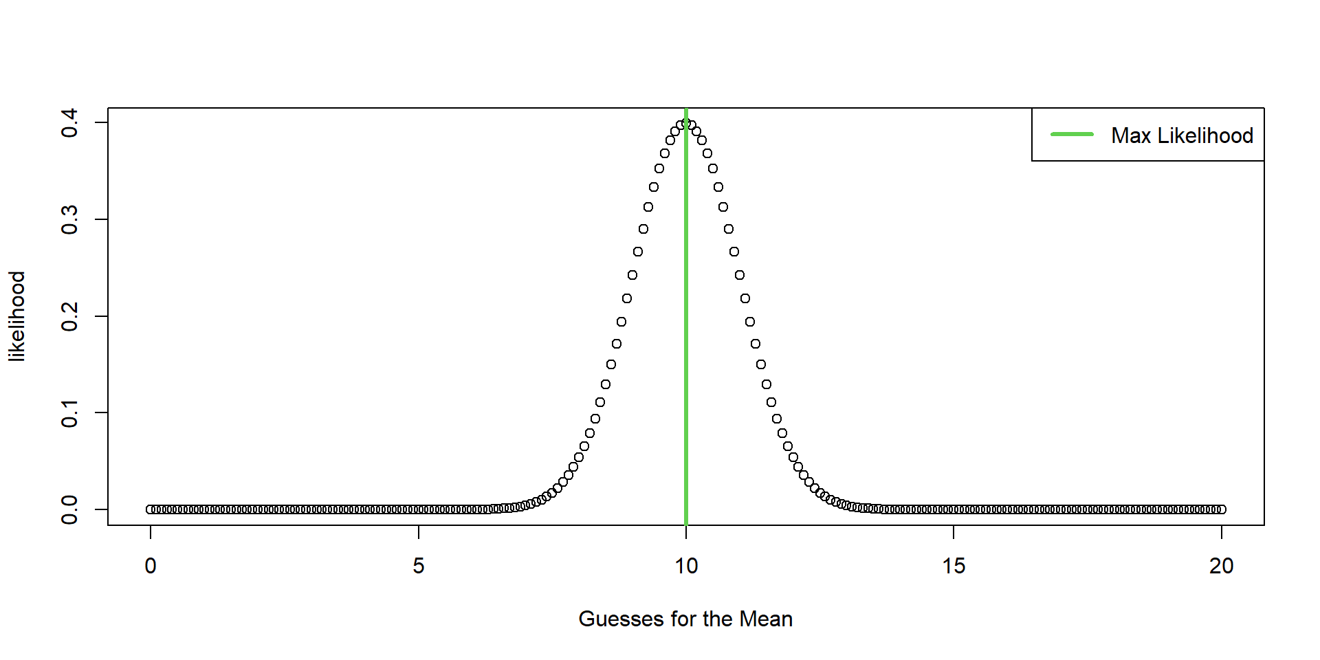
If we knew the mean is truly 8, it would also be the probability density of the observation y = 10. But, we don’t know what the mean truly is.
The key is to understand that the likelihood values are relative, which means we need many guesses.
Optimization
Grid Search
Maximum Likelihood Properties
Central Tenet: evidence is relative.
Parameters are not RVs. They are not defined by a PDF/PMF.
MLEs are consistent. As sample size increases, they will converge to the true parameter value.
MLEs are asymptotically unbiased. The \(E[\hat{\theta}]\) converges to \(\theta\) as the sample size gets larger.
No guarantee that MLE is unbiased at small sample size. Can be tested!
MLEs will have the minimum variance among all estimators, as the sample size gets larger.
MLE with n > 1
What is the mean height of King Penguins?
MLE with n > 1
We go and collect data,
\(\boldsymbol{y} = \begin{matrix} [4.34 & 3.53 & 3.75] \end{matrix}\)
Let’s decide to use the Normal Distribution as our PDF.
\[ \begin{align*} f(y_1 = 4.34|\mu,\sigma) &= \frac{1}{\sigma\sqrt(2\pi)}e^{-\frac{1}{2}(\frac{y_{1}-\mu}{\sigma})^2} \\ \end{align*} \]
AND
\[ \begin{align*} f(y_2 = 3.53|\mu,\sigma) &= \frac{1}{\sigma\sqrt(2\pi)}e^{-\frac{1}{2}(\frac{y_{2}-\mu}{\sigma})^2} \\ \end{align*} \]
AND
\[ \begin{align*} f(y_3 = 3.75|\mu,\sigma) &= \frac{1}{\sigma\sqrt(2\pi)}e^{-\frac{1}{2}(\frac{y_{3}-\mu}{\sigma})^2} \\ \end{align*} \]
Need to connect data together
Or simply,
\[ \textbf{y} \stackrel{iid}{\sim} \text{Normal}(\mu, \sigma) \]
\(iid\) = independent and identically distributed
Need to connect data together
The joint probability of our data with shared parameters \(\mu\) and \(\sigma\),
\[ \begin{align*} & P(Y_{1} = y_1,Y_{2} = y_2, Y_{3} = y_3 | \mu, \sigma) \\ \end{align*} \]
\[ \begin{align*} & P(Y_{1} = 4.34,Y_{2} = 3.53, Y_{3} = 3.75 | \mu, \sigma) \\ &= \mathcal{L}(\mu, \sigma|\textbf{y}) \end{align*} \]
Need to connect data together
IF each \(y_{i}\) is independent, the joint probability of our data are simply the multiplication of all three probability densities,
\[ \begin{align*} =& f(4.34|\mu, \sigma)\times f(3.53|\mu, \sigma)\times f(3.75|\mu, \sigma) \end{align*} \] \[ \begin{align*} =& \prod_{i=1}^{3} f(y_{i}|\mu, \sigma) \\ =& \mathcal{L}(\mu, \sigma|y_{1},y_{2},y_{3}) \end{align*} \]
Conditional Independence Assumption
We can do this because we are assuming knowing one observation does not tell us any new information about another observation. Such that,
\(P(y_{2}|y_{1}) = P(y_{2})\)
Code
Translate the math to code…
Optimization Code (Grid Search)
Calculate likelihood of many guesses of \(\mu\) and \(\sigma\) simultaneously,
MLE Code
Likelihood plot (3D)
Sample Size
What happens to the likelihood if we increase the sample size to N=100?