   y  veg effort
1 15 Veg1      5
2 18 Veg1      5
3 12 Veg2      5
4 14 Veg2      5
5 12 Veg2      5
6 14 Veg2      5
Veg1 Veg2 Veg3 Veg4 Veg5
2 20 20 10 10 Study goals
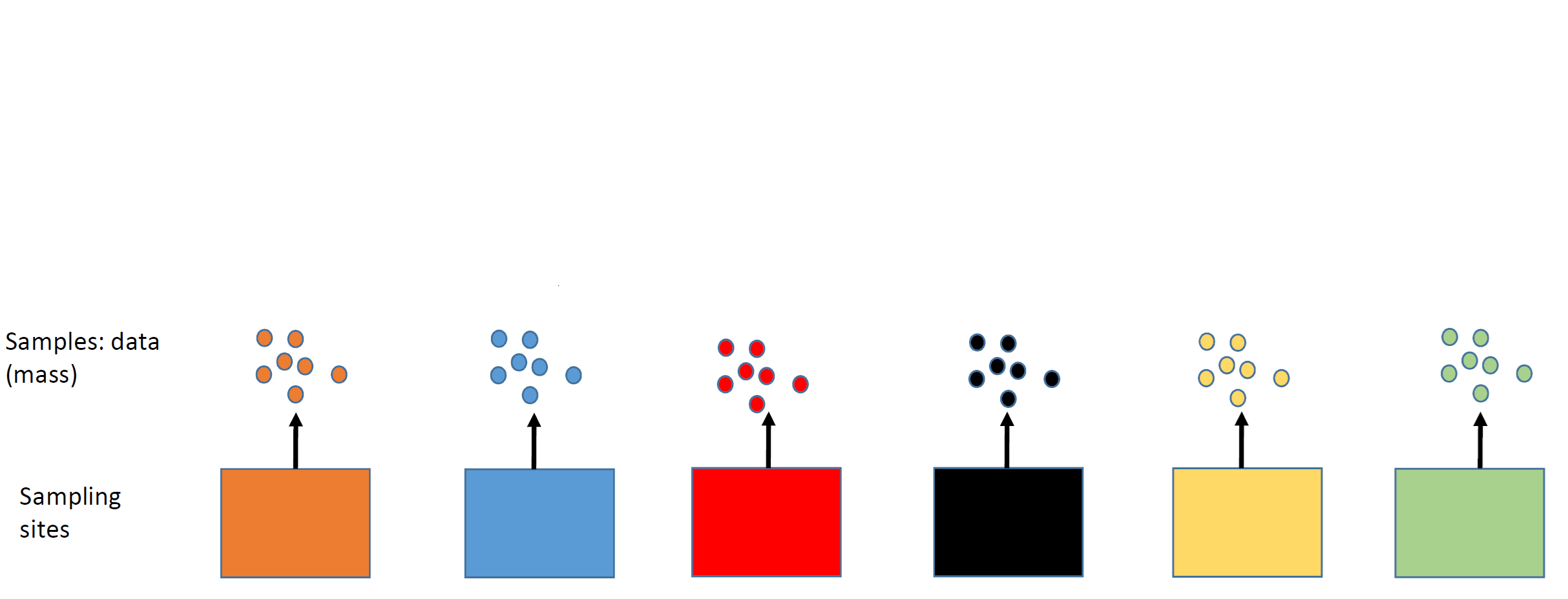
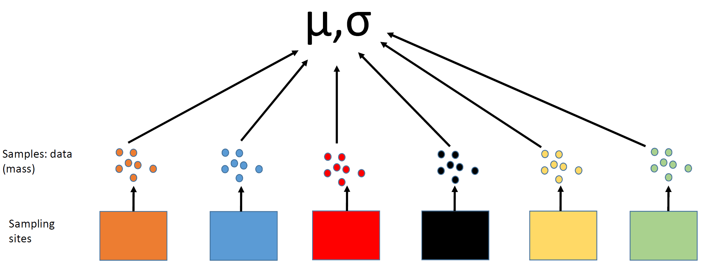
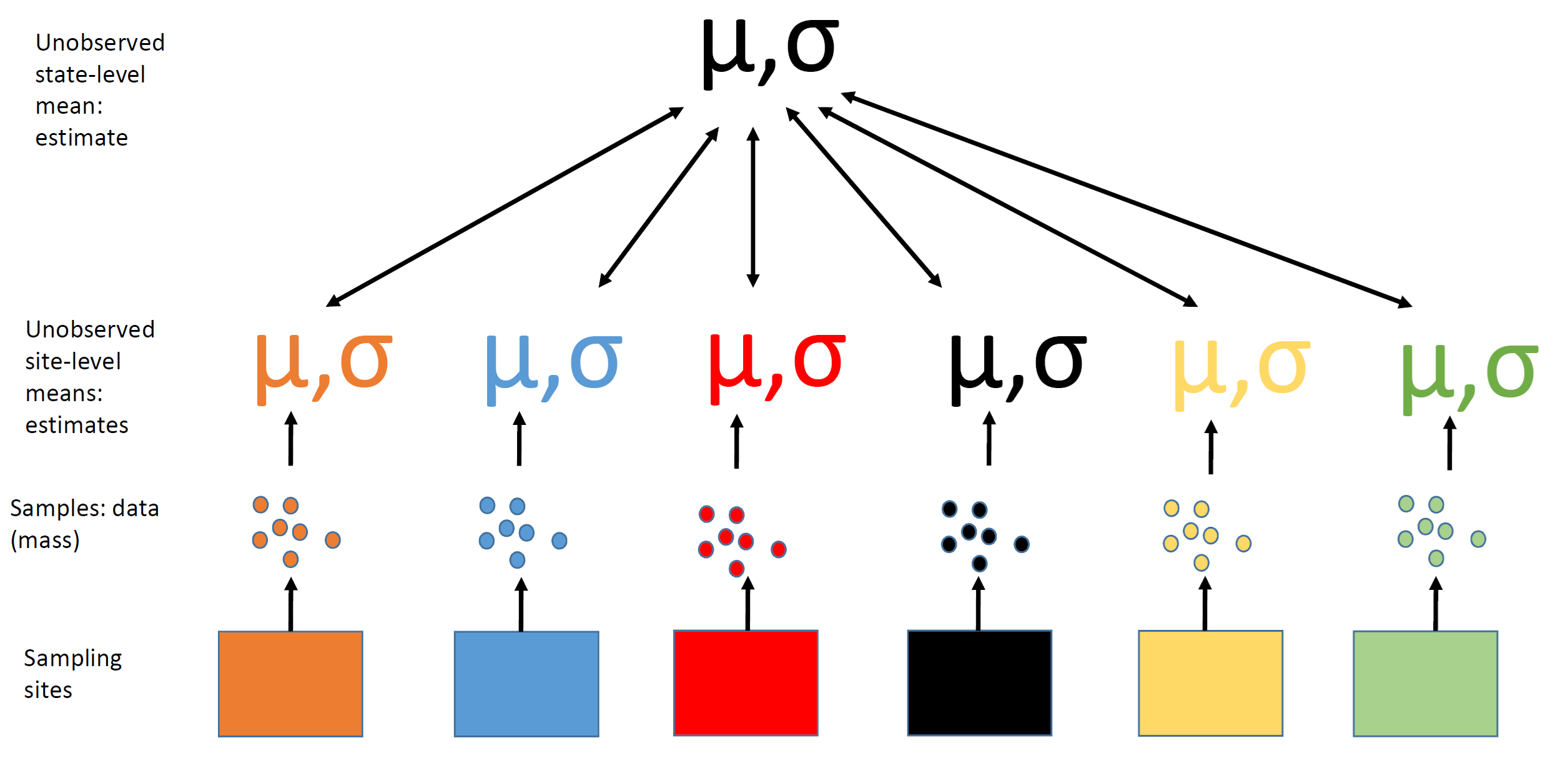
Estimate state-wide average mass
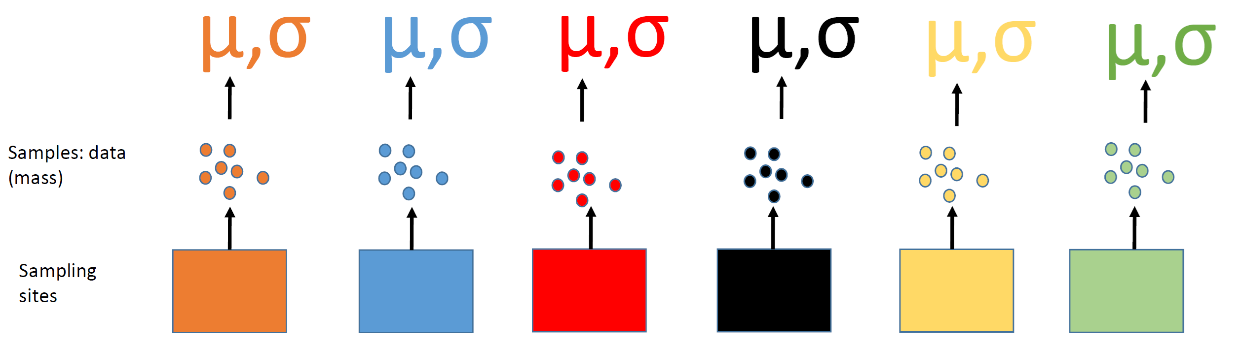
Understand site-level variation
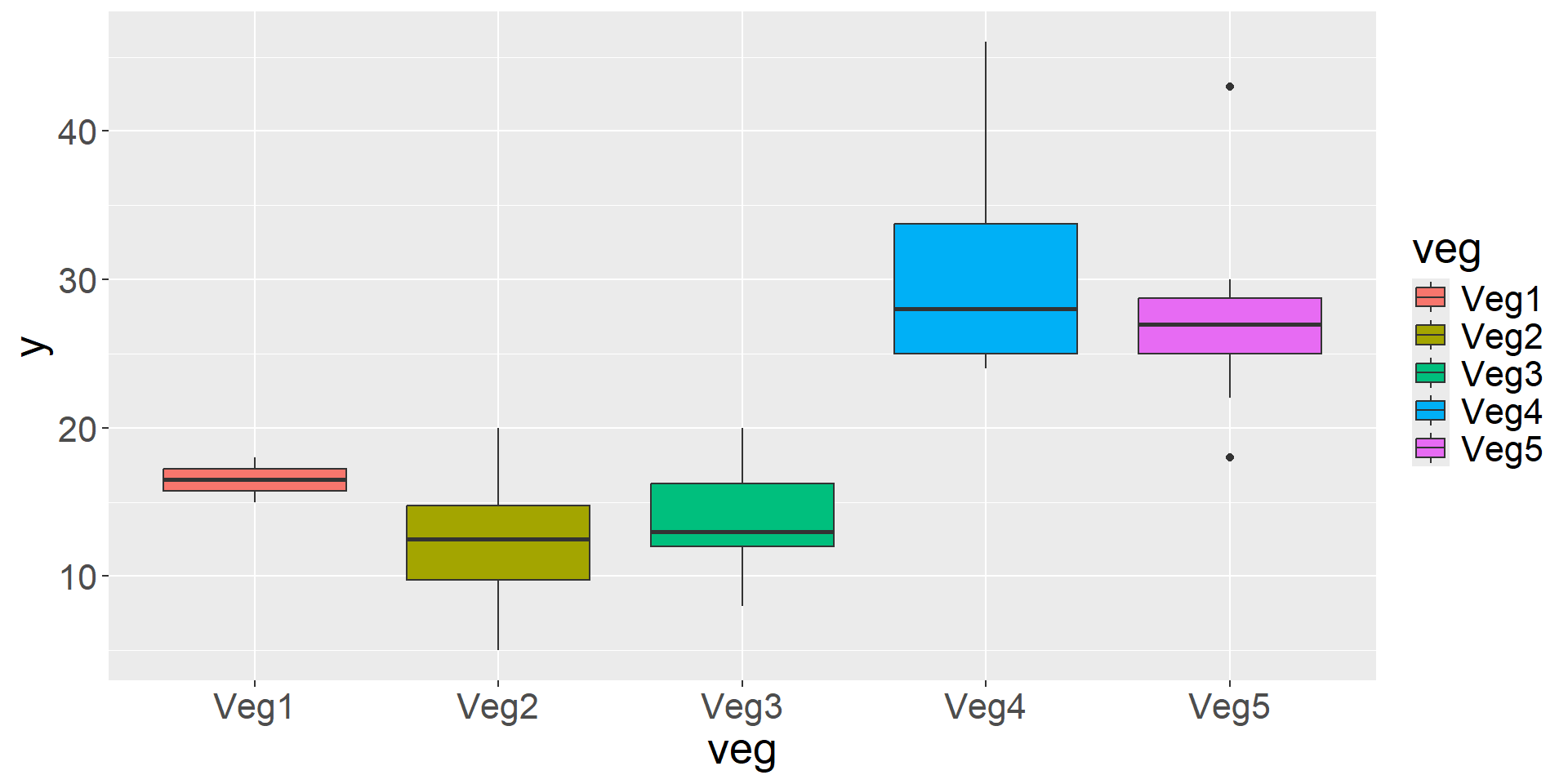
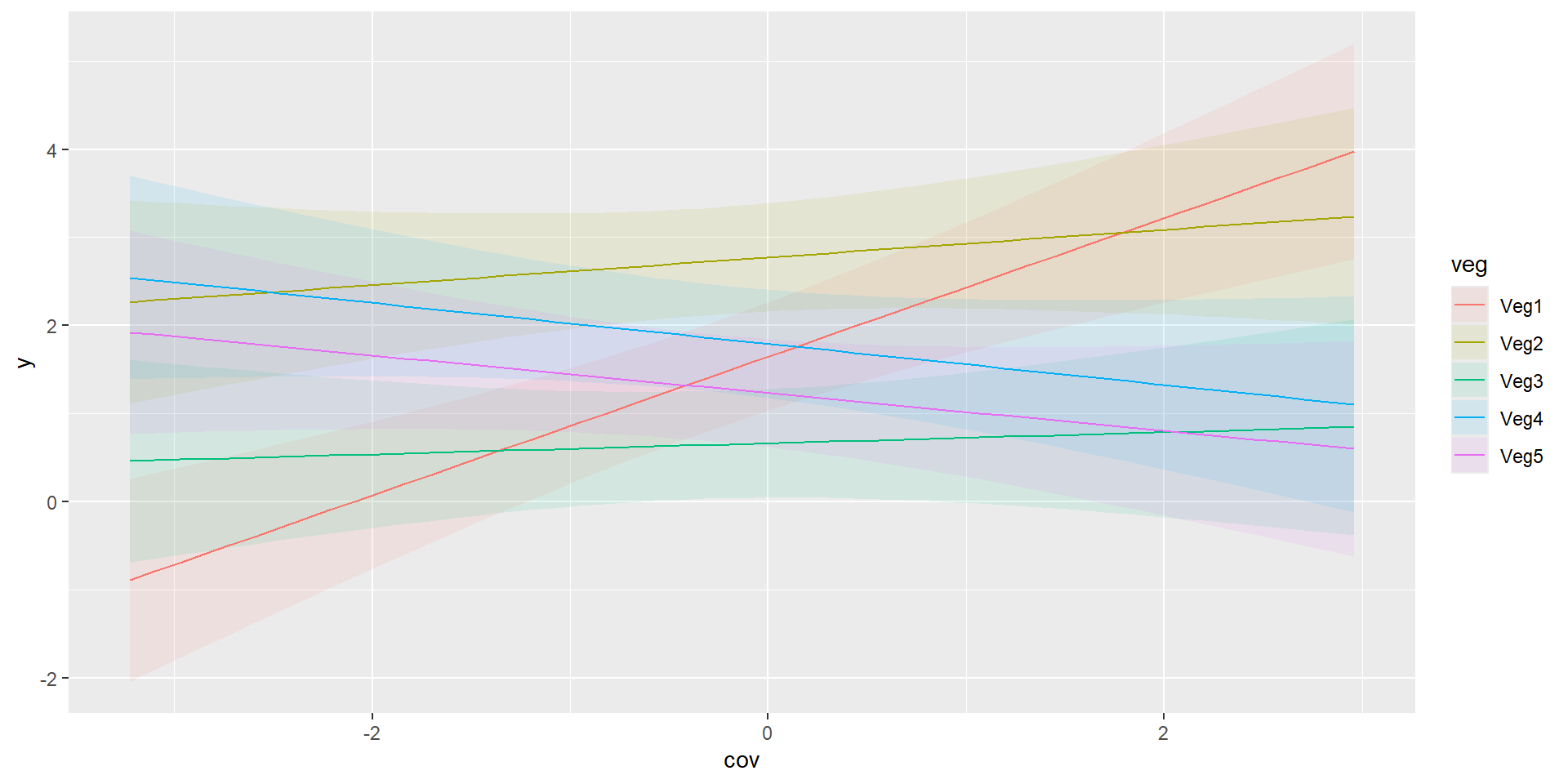
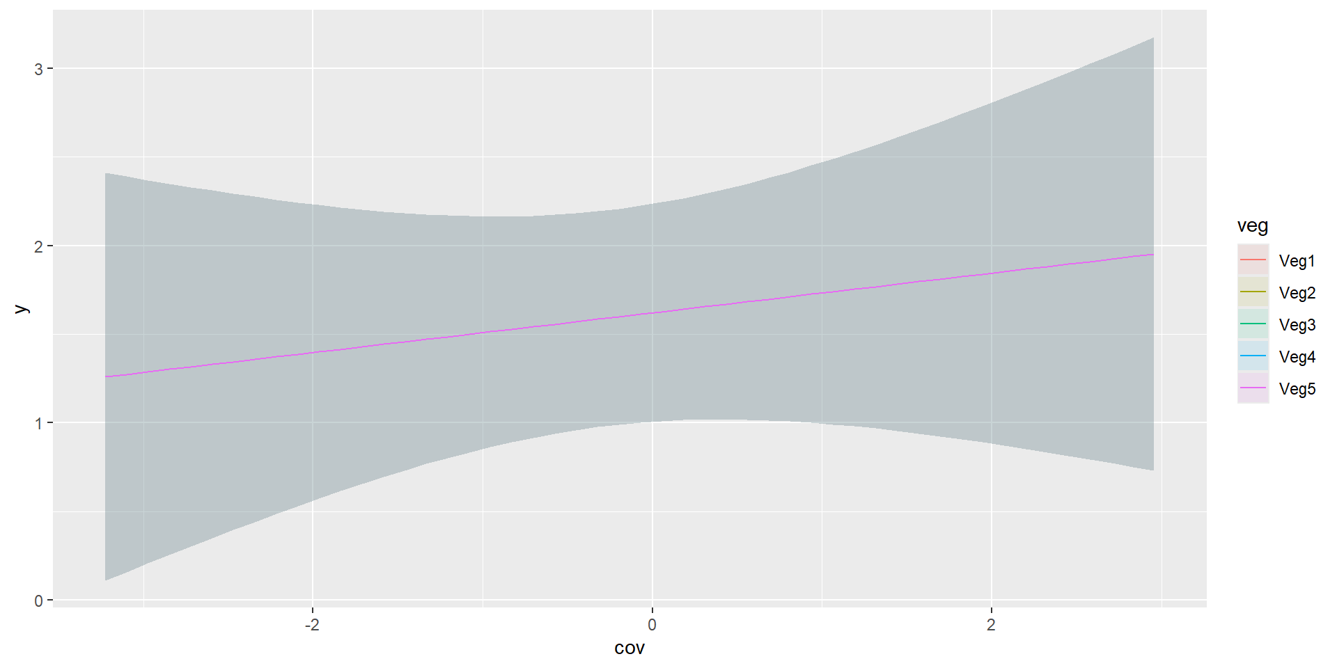
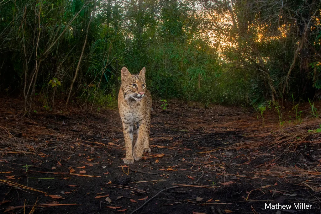
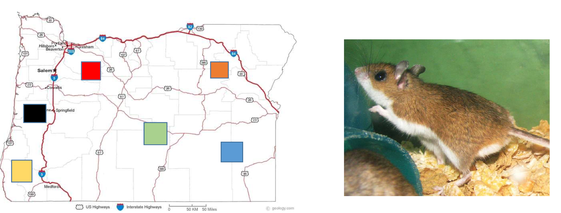
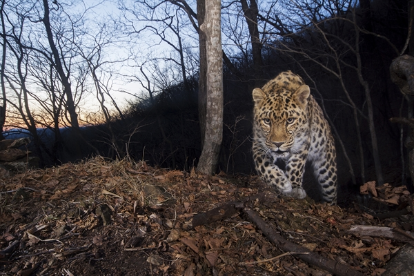
We sample Amur Leopards in five different vegetation types of Land of the Leopard National Park.
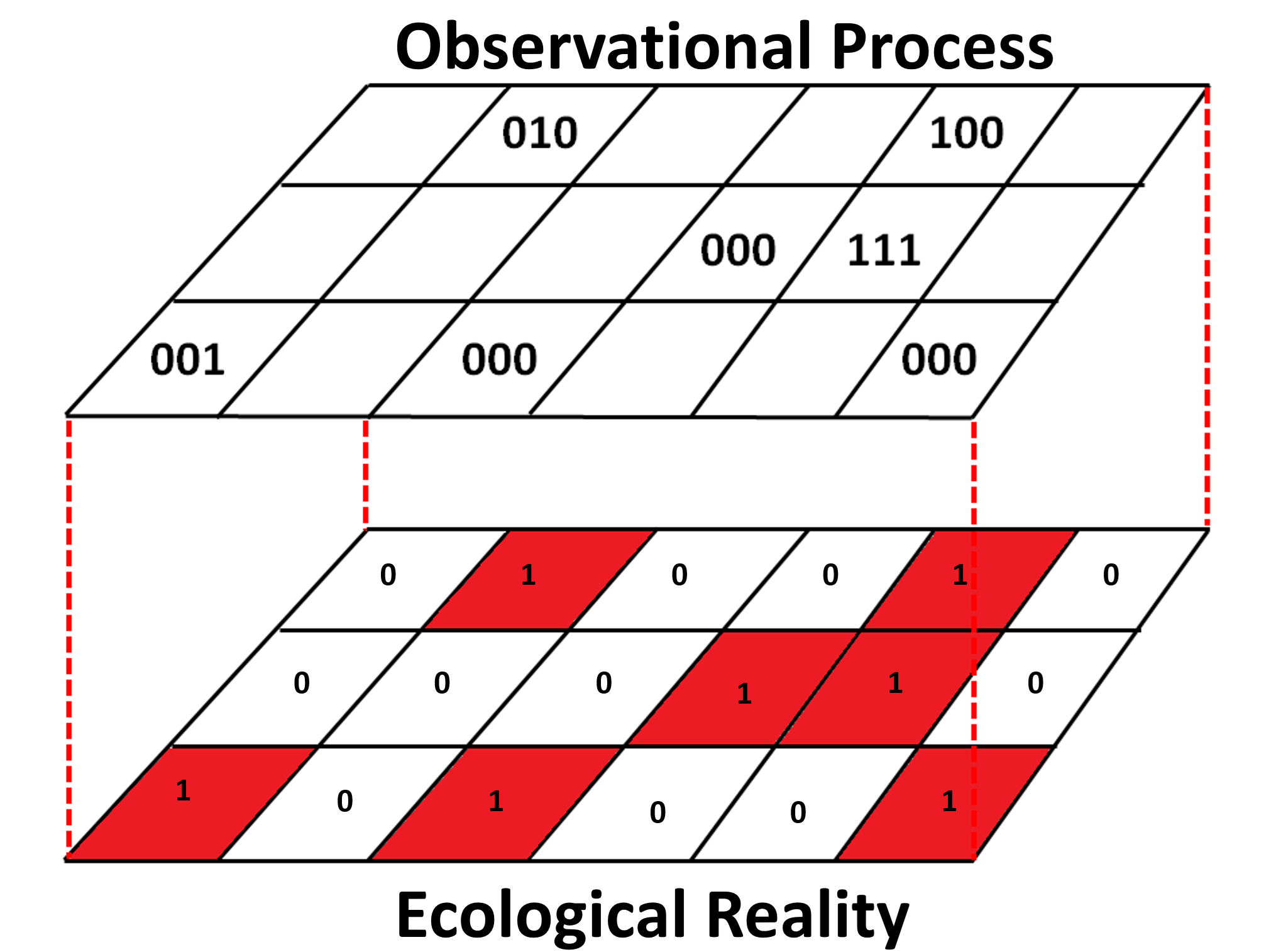
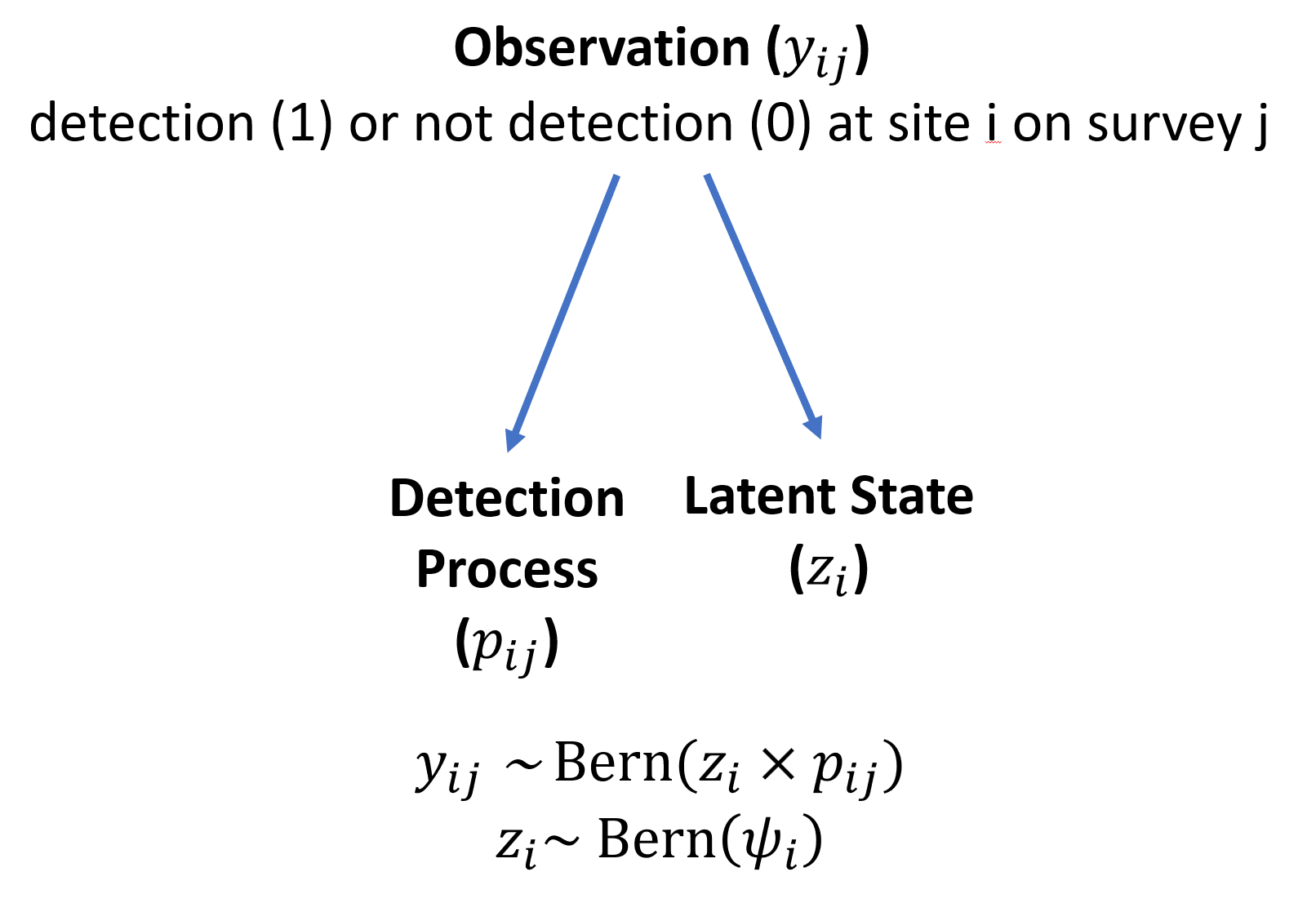
Interested in detection rate by vegetation type and overall.
We sample Amur Leopards in five different vegetation types of Land of the Leopard National Park.
Detection Rate = Independent Counts / Effort
y veg effort
1 15 Veg1 5
2 18 Veg1 5
3 12 Veg2 5
4 14 Veg2 5
5 12 Veg2 5
6 14 Veg2 5
Veg1 Veg2 Veg3 Veg4 Veg5
2 20 20 10 10