Generalized Linear Models

Objectives

• GLM framework
• matrix notation
• linear algebra
• design matrix / categorical variable
• glm function
• link functions
• logistic regression

GLM

Generalized linear model framework using matrix notation

\[ \begin{align*} \textbf{y}\sim& [\textbf{y}|\boldsymbol{\mu},\sigma] \\ \text{g}(\boldsymbol{\mu}) =& \textbf{X}\boldsymbol{\beta} \end{align*} \]

Motivation

GLMs:

• t-test
• ANOVA/ANCOVA
• linear regression
• logistic / probit regression
• Poisson regression
• log-linear regression
• survival analysis
• AND MORE!

GLM

Generalized linear model framework

\[ \begin{align*} \textbf{y}\sim& [\textbf{y}|\boldsymbol{\mu},\sigma] \\ \text{g}(\boldsymbol{\mu}) =& \textbf{X}\boldsymbol{\beta} \end{align*} \]

Elements

• prob. function to define the RV (\(\textbf{y}\))

• parameters or moments of the prob. function (\(\boldsymbol{\mu},\sigma\))

• link function (\(\text{g}(\boldsymbol{\mu})\)); deterministic transformation of parameters to new scale

• inverse-link function (\(\text{g}^{-1}(\boldsymbol{\textbf{X}\boldsymbol{\beta}})\)); deterministic transformation of linear combination back to parameter scale

• design matrix of the explanatory variables (\(\textbf{X}\)); these are known

• coefficient parameters (\(\boldsymbol{\beta}\)); needs estimating

Linear Regression

index notation

\[ \begin{align*} y_{i} \sim& \text{Normal}(\mu_{i},\sigma) \\ \mu_{i} =& \beta_{0} + \beta_{1}x_{1i} + \beta_{2}x_{2i} \end{align*} \]

matrix notation

\[ \begin{align*} \textbf{y}\sim& \text{Normal}(\boldsymbol{\mu},\sigma)\\ \boldsymbol{\mu} =& \text{g}^{-1}(\textbf{X}\boldsymbol{\beta})\\ \text{g}(\boldsymbol{\mu}) =& \textbf{X}\boldsymbol{\beta} \end{align*} \]

\[\begin{align*} \textbf{y} = \begin{bmatrix} y_{1} \\ y_{2} \\ y_{3} \\ . \\ . \\ y_{n} \end{bmatrix} \textbf{X} = \begin{bmatrix} 1 & x_{1,2} & x_{1,3} \\ 1 & x_{2,2} & x_{2,3} \\ 1 & x_{3,2} & x_{3,3} \\ . & . .\\ . & . .\\ n & x_{n,2} & x_{n,3} \end{bmatrix} \boldsymbol{\beta} = \begin{bmatrix} \beta_0 \\ \beta_1 \\ \beta_2 \\ \end{bmatrix} \end{align*}\]

n = sample size x\(_{2}\) & x\(_{3}\) are independent variables

Linear Algebra

\(\text{g}(\boldsymbol{\mu}) = \textbf{X}\boldsymbol{\beta}\)

\(\textbf{X}\) is called the Design Matrix.

\(\boldsymbol{\beta}\) is a vector of coefficients.

\[ \textbf{X}= \begin{bmatrix} 1 & x_{1,2} & x_{1,3} \\ 1 & x_{2,2} & x_{2,3} \\ 1 & x_{3,2} & x_{3,3} \end{bmatrix} \boldsymbol{\beta} = \begin{bmatrix} \beta_0 \\ \beta_1 \\ \beta_2 \end{bmatrix} \]

\[ \textbf{X}\boldsymbol{\beta} = \begin{bmatrix} \beta_0\times 1 + \beta_1\times x_{1,2} + \beta_2\times x_{1,3} \\ \beta_0\times 1 + \beta_1\times x_{2,2} + \beta_2\times x_{2,3} \\ \beta_0\times 1 + \beta_1\times x_{3,2} + \beta_2\times x_{3,3} \\ \end{bmatrix}\\ \]

\[ \textbf{X}\boldsymbol{\beta} = \begin{bmatrix} \beta_0 + \beta_1 x_{1,2} + \beta_2 x_{1,3} \\ \beta_0 + \beta_1 x_{2,2} + \beta_2 x_{2,3} \\ \beta_0 + \beta_1 x_{3,2} + \beta_2 x_{3,3} \\ \end{bmatrix}\\ \]

\[ \text{g}(\boldsymbol{\mu}) = \textbf{X}\boldsymbol{\beta} = \begin{bmatrix} \text{lt}_{1} \\ \text{lt}_{2} \\ \text{lt}_{3} \end{bmatrix} \] lt = linear terms

\[ \boldsymbol{\mu} = \text{g}^{-1}(\textbf{X}\boldsymbol{\beta})\ = \textbf{X}\boldsymbol{\beta} / 1= \begin{bmatrix} \text{lt}_{1}/1 \\ \text{lt}_{2}/1 \\ \text{lt}_{3}/1 \end{bmatrix} \]

\[ \boldsymbol{\mu} = \textbf{X}\boldsymbol{\beta} = \begin{bmatrix} \mu_{1} \\ \mu_{2} \\ \mu_{3} \end{bmatrix} \]

Linear Algebra

• \(\textbf{y}'\textbf{y}\)

• \(\textbf{y}' \cdot \textbf{y}\)

\[ =\begin{bmatrix} 1 & 2 & 3 \end{bmatrix} \begin{bmatrix} 1 \\ 2 \\ 3 \\ \end{bmatrix} \]

\[ =\begin{bmatrix} (1\times1) + (2\times2) + (3\times3)\\ \end{bmatrix} \\= [14] \]

y <- matrix(c(1,2,3),nrow=3,ncol=1)
t(y)%*%y

     [,1]
[1,]   14

Linear Algebra

When can we do matrix multiplication?

first=t(y)
dim(first)

[1] 1 3

second=y
dim(second)

[1] 3 1

#When this is true
  ncol(first)==nrow(second)

[1] TRUE

(1 x 3) (3 x 1)

Linear Algebra

Note that

\(\textbf{y}'\textbf{y} \neq \textbf{y}\textbf{y}'\)

t(y)%*%y

     [,1]
[1,]   14

y%*%t(y)

     [,1] [,2] [,3]
[1,]    1    2    3
[2,]    2    4    6
[3,]    3    6    9

Elephant Linear Regression Example

Categorical Variable

     weight    sex
1 11488.991   Male
2  4105.442 Female
3  4299.308 Female

Elephant Linear Regression Example

Categorical Variable

model = glm(weight~sex, 
            data=dat,
            family=gaussian(link = identity)
            )
summary(model)

Call:
glm(formula = weight ~ sex, family = gaussian(link = identity), 
    data = dat)

Coefficients:
            Estimate Std. Error t value Pr(>|t|)    
(Intercept)   4970.9      120.9   41.11   <2e-16 ***
sexMale       6848.1      180.2   37.99   <2e-16 ***
---
Signif. codes:  0 '***' 0.001 '**' 0.01 '*' 0.05 '.' 0.1 ' ' 1

(Dispersion parameter for gaussian family taken to be 1608053)

    Null deviance: 2639772182  on 199  degrees of freedom
Residual deviance:  318394574  on 198  degrees of freedom
AIC: 3429.7

Number of Fisher Scoring iterations: 2

Elephant Linear Regression Example

Categorical Variable

\(x_{2}\) as an indicator of sex, female (0) or male (1)

\(x_{3}\) elephant age

\[ \textbf{weight} \sim \text{Normal}(\boldsymbol{\mu},\sigma)\\ \\ \boldsymbol{\mu} =\textbf{X}\boldsymbol{\beta} = \begin{bmatrix} \beta_0 + (\beta_1\times 1) + (\beta_2\times 10) \\ \beta_0 + (\beta_1\times 0) + (\beta_2\times 12) \\ \beta_0 + (\beta_1\times 0) + (\beta_2\times 15) \\ \end{bmatrix}\\ \]

\[ \hat{\boldsymbol{\mu}} = \textbf{X}\hat{\boldsymbol{\beta}} = \begin{bmatrix} 2552.82 + (6828.96\times 1) + (145.74\times 10) \\ 2552.82 + (6828.96\times 0) + (145.74\times 12) \\ 2552.82 + (6828.96\times 0) + (145.74\times 15) \\ \end{bmatrix}\\ \]

\[ \hat{\boldsymbol{\mu}} = \textbf{X}\hat{\boldsymbol{\beta}} = \begin{bmatrix} 2552.82 + 6828.96 + 1457.4 \\ 2552.82 + 0 + 1748.88 \\ 2552.82 + 0 + 2186.1 \\ \end{bmatrix}\\ \]

\[ \hat{\boldsymbol{\mu}} = \textbf{X}\hat{\boldsymbol{\beta}} = \begin{bmatrix} 10401.98 \\ 6779.52 \\ 5322.02 \\ \end{bmatrix}\\ \]

So, what does \(\beta_1\) mean?

glm and design matix

# GLM coefs
  X = model.matrix(~sex+age.years,data=dat)
  head(X)

  (Intercept) sexMale age.years
1           1       1        10
2           1       0        12
3           1       0        15
4           1       0        12
5           1       1        20
6           1       1         4

  glm(weight~0+X,data=dat)

Call:  glm(formula = weight ~ 0 + X, data = dat)

Coefficients:
X(Intercept)      XsexMale    Xage.years  
      2552.8        6829.0         145.7  

Degrees of Freedom: 200 Total (i.e. Null);  197 Residual
Null Deviance:      1.561e+10 
Residual Deviance: 75320000     AIC: 3143

Sex variable is arranged by ‘Dummy Coding’

MLE Estimator with Linear Algebra

\[ \hat{\boldsymbol{\beta}} = (\textbf{X}'\textbf{X})^{-1}\textbf{X}'\textbf{y} \]

X(Intercept)     XsexMale   Xage.years 
   2552.8203    6828.9645     145.7483 

# Linear Algebra Maximum Likelihood Estimate
  y=dat$weight
  c(solve(t(X)%*%X)%*%t(X)%*%y)

[1] 2552.8203 6828.9645  145.7483

Link functions

• \(\text{g}(\boldsymbol{\mu}) = \textbf{X}\boldsymbol{\beta}\)

• \(\boldsymbol{\mu} = \text{g}^{-1}(\textbf{X}\boldsymbol{\beta})\)

Link functions map parameters from one support to another.

Why is that important for us?

To put a linear model on parameters of interest and ensure the parameter support is maintained.

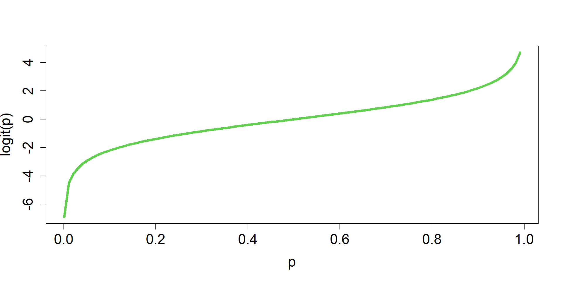
Computers do not like boundaries (e.g., 0 or 1). It’s easier to guess values to evaluate in a maximum liklihood optimization when there are no bounds. (\(-\infty\), \(\infty\))

Link functions

Identity

No transformation is needed because the parameter support is maintained. \[ \begin{align*} \boldsymbol{\mu} \in& (-\infty,\infty)\\ \textbf{X}\boldsymbol{\beta} \in& (-\infty,\infty) \end{align*} \]

A Model by another name

Model Name	\([y|\boldsymbol{\theta}]\)	Link
ANOVA (\(x_{1}\) is categorical/multiple levels)	Normal	identity
ANCOVA (\(x_{1}\) is categorical, \(x_{2}\) is continuous))	Normal	identity
t-test (\(x_{1}\) is categorical with 2 levels)	Normal	identity
Linear Regression \(x_{1}\) is continuous	Normal	identity
Multiple Linear Regression \(x_{p}\) is continuous	Normal	identity
Logistic Regression	Binomial	logit
Probit Regression	Binomial	probit
Log-linear Regression	Poisson	log
Poisson Regression	Poisson	log
Survival Analysis	Exponential	log
Inverse Polynomial	Gamma	Reciprocal

Nelder and Wedderburn (1972)

Logistic Regression (logit link)

\[ \begin{align*} \textbf{y} \sim& \text{Binomial}(N,\boldsymbol{p}) \end{align*} \]

\[ \begin{align*} \text{g}(\boldsymbol{p}) =& \text{logit}(\boldsymbol{p}) = \text{log}(\frac{\boldsymbol{p}}{1-\boldsymbol{p}}) \end{align*} \]

inverse-logit (expit)

\[ \boldsymbol{p} = g^{-1}(\boldsymbol{\textbf{X}\boldsymbol{\beta}}) = \text{logit}^{-1}(\textbf{X}\boldsymbol{\beta}) = \frac{e^{\textbf{X}\boldsymbol{\beta}}}{e^{\textbf{X}\boldsymbol{\beta}}+1} \]

Logistic Regression

Full model

\[ \begin{align*} \textbf{y} \sim& \text{Binomial}(N,\boldsymbol{p})\\ \text{logit}(\boldsymbol{p}) =& \textbf{X}\boldsymbol{\beta} \end{align*} \]

Remember,
\(\boldsymbol{p} \in [0,1]\)

\(\textbf{X}\boldsymbol{\beta} \in (-\infty,\infty)\)

logit/p mapping

p=seq(0.001,0.999,by=0.01)
logit.p=qlogis(p)
par(cex.lab=1.5,cex.axis=1.5)
plot(p,logit.p,type="l",lwd=4,col=3,xlab='p',ylab="logit(p)")

Logistic Regression Simulation

#Design matrix
  set.seed(43534)
  Var1 = rnorm(100)
  X = model.matrix(~Var1)
  head(X)

  (Intercept)       Var1
1           1  1.4371396
2           1 -0.4835090
3           1  1.0370452
4           1 -0.5894099
5           1  1.2633564
6           1 -1.9008071

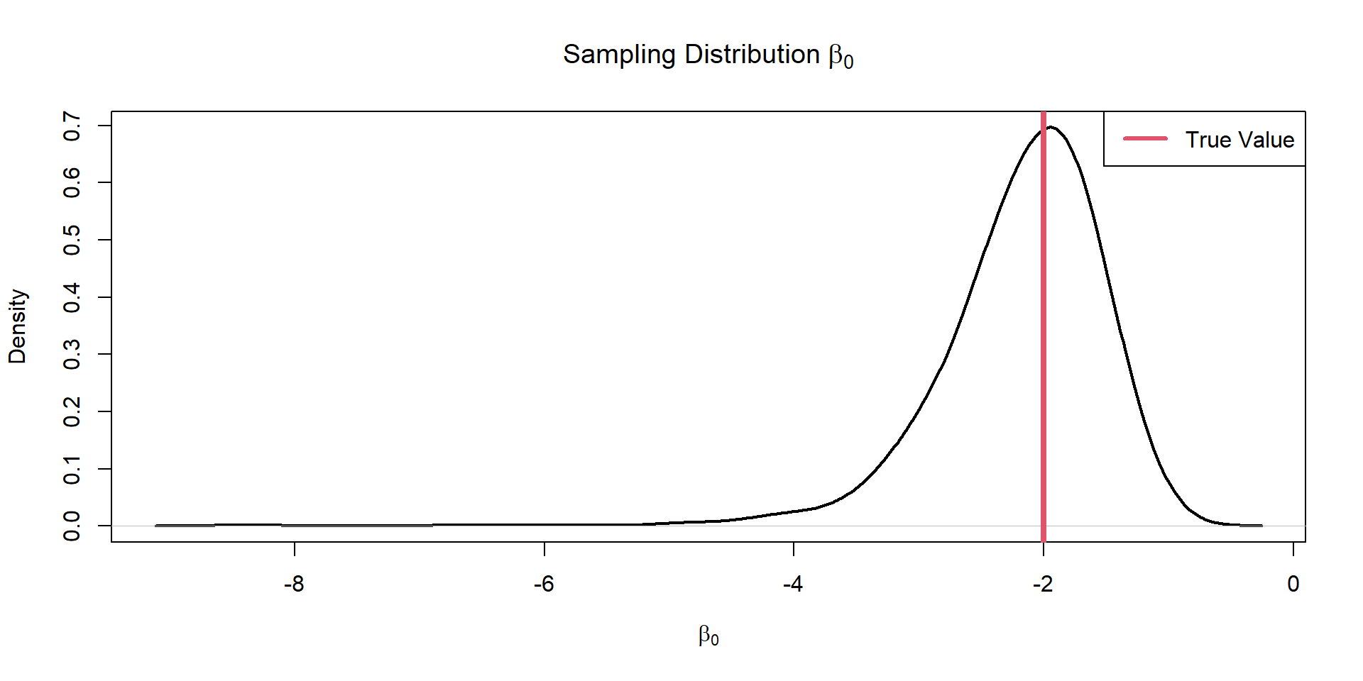
# marginal coefficients (on logit-scale)
  beta=c(-2,4)

#linear terms
  lt = X%*%beta

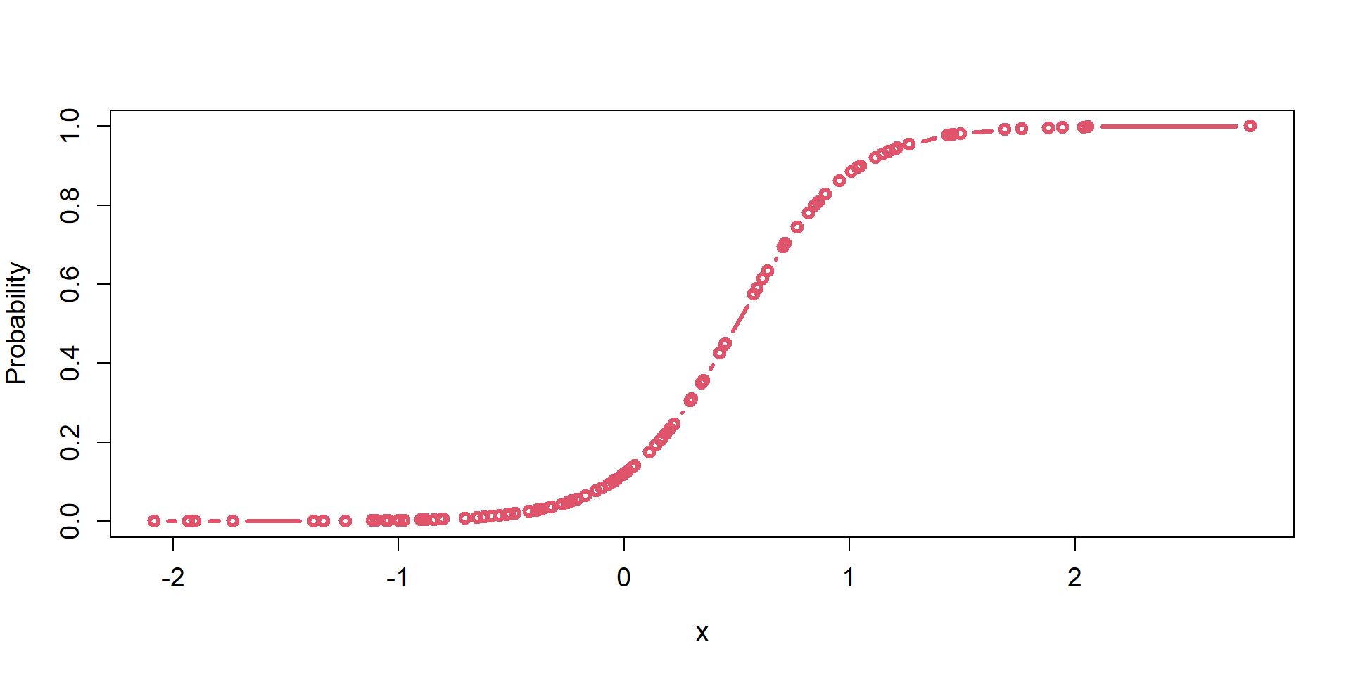
#transformation via link function to probability scale
  p=plogis(lt)
  head(round(p,digits=2))

  [,1]
1 0.98
2 0.02
3 0.90
4 0.01
5 0.95
6 0.00

#sample
  set.seed(14353)
  y = rbinom(n=length(p),size=1,p)
  y

  [1] 1 0 1 0 1 0 0 1 0 1 0 0 0 1 1 0 0 1 1 0 0 1 0 0 0 0 0 0 0 0 0 1 1 0 0 0 0
 [38] 0 1 1 0 1 0 1 0 1 1 0 1 1 1 1 0 0 1 1 0 1 0 1 0 1 1 0 0 0 0 0 0 0 0 0 0 0
 [75] 0 0 0 0 0 1 1 0 0 1 0 0 0 0 1 1 0 0 1 0 0 0 0 0 1 0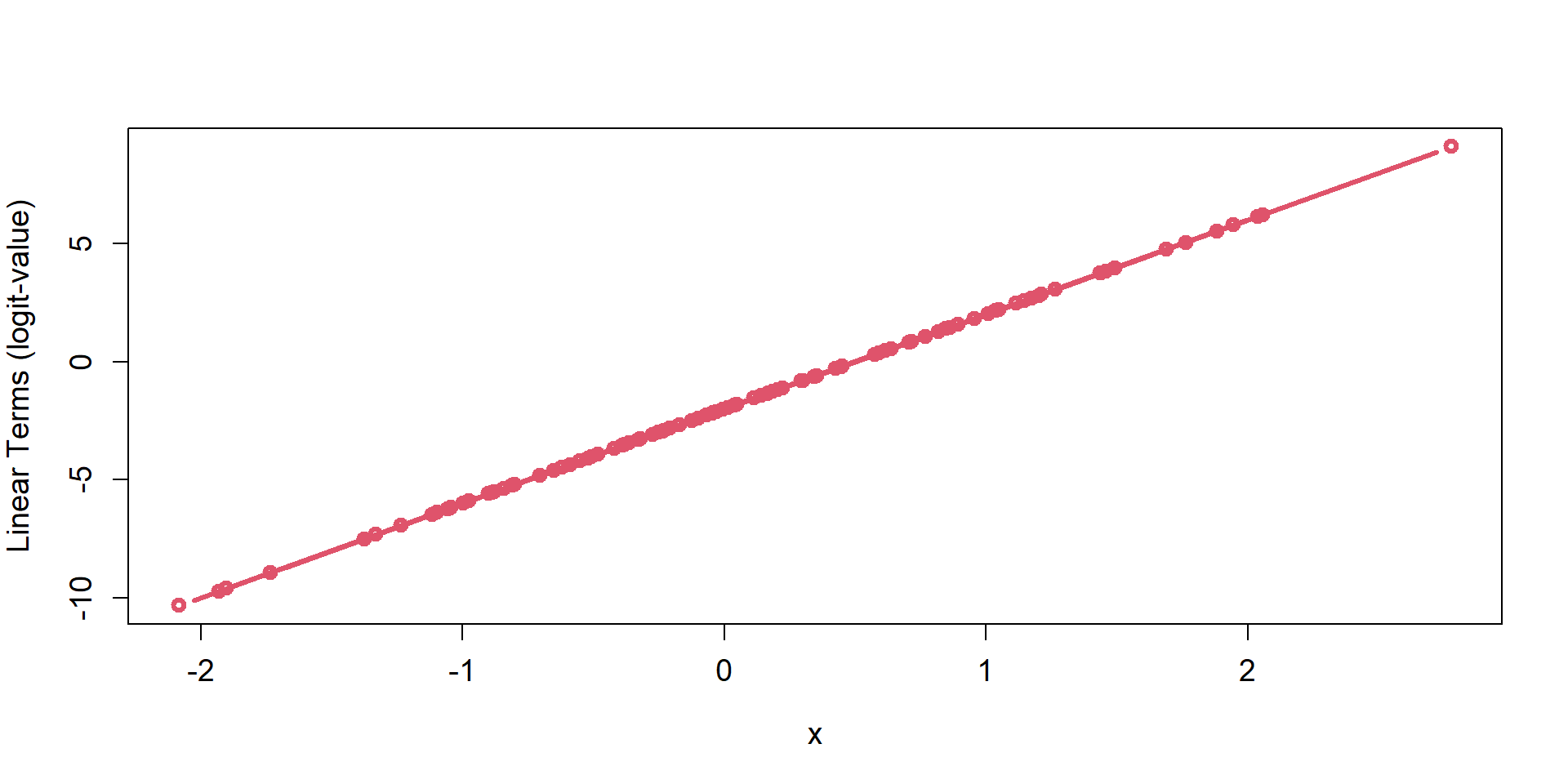

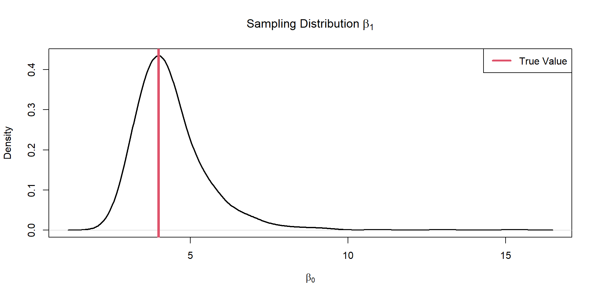
#Plot the linear 'terms'  and explantory variable
  par(cex.lab=1.2,cex.axis=1.2)
  plot(Var1,lt,type="b",lwd=3,col=2,
       xlab="x",ylab="Linear Terms (logit-value)")  

  index=order(Var1)
  plot(Var1[index],p[index],type="b",lwd=3,col=2,xlab="x",ylab="Probability")  

Logistic Regression Estimation

# Fit model to sample 
  model1=glm(y~0+X, family = binomial(link = "logit"))
  summary(model1)

Call:
glm(formula = y ~ 0 + X, family = binomial(link = "logit"))

Coefficients:
             Estimate Std. Error z value Pr(>|z|)    
X(Intercept)  -2.5304     0.6473  -3.909 9.25e-05 ***
XVar1          5.4198     1.2232   4.431 9.38e-06 ***
---
Signif. codes:  0 '***' 0.001 '**' 0.01 '*' 0.05 '.' 0.1 ' ' 1

(Dispersion parameter for binomial family taken to be 1)

    Null deviance: 138.63  on 100  degrees of freedom
Residual deviance:  39.14  on  98  degrees of freedom
AIC: 43.14

Number of Fisher Scoring iterations: 7

Logistic Regression Evaluation

 #sample many times  
  n.sim=1000
  y.many = replicate(n.sim,rbinom(n=length(p),size=1,p))
  dim(y.many)

[1]  100 1000

 #Estimate coefs for all 100 samples
  coef.est=apply(y.many,2,FUN=function(y){
          model1=glm(y~0+X, family = binomial(link = "logit"))
          
  model1$coefficients
  })

  dim(coef.est)

[1]    2 1000

Plot Intercept

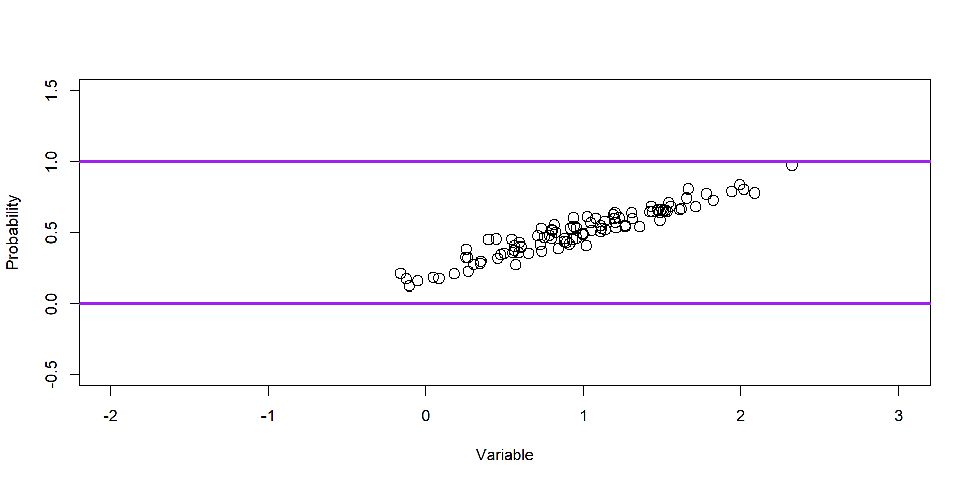
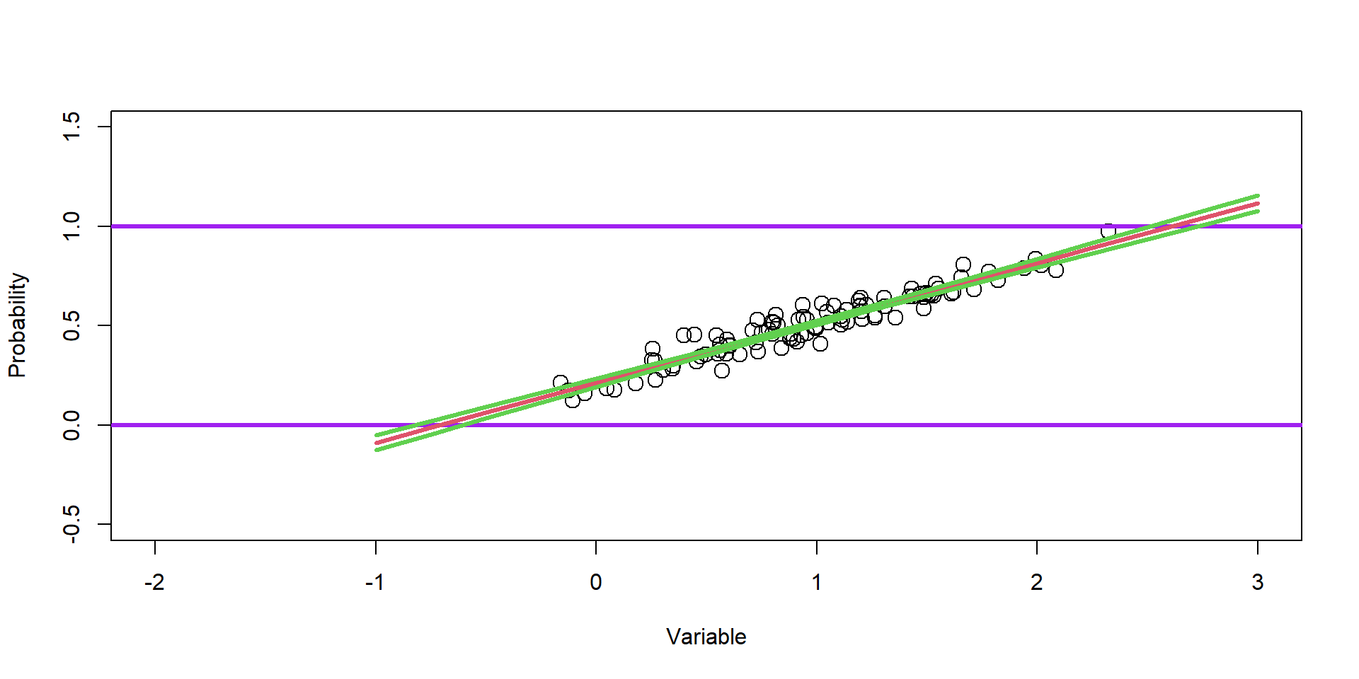
Plot Slope

Evaluate Sampling Distributions

Is our model biased?

# Relative Bias
  (mean(coef.est[1,])-beta[1])/beta[1]

[1] 0.0879452

  (mean(coef.est[2,])-beta[2])/beta[2]

[1] 0.09751027

Evaluate Sampling Distributions

Are we going to estimate the sign of the coef correctly?

# Probability of estimating a coef sign correctly
  length(which(coef.est[1,]<0))/n.sim

[1] 1

  length(which(coef.est[2,]>0))/n.sim

[1] 1

Logistic Regression Biased Correction

brglm: Bias Reduction in Binomial-Response Generalized Linear Models

brglm::brglm(y~0+X, family = binomial(link = "logit"))

# Relative Bias
  (mean(coef.est[1,])-beta[1])/beta[1]

[1] 0.007785692

  (mean(coef.est[2,])-beta[2])/beta[2]

[1] 0.008799186

Recap

• GLM framework: What are key components?
• matrix notation - why learn this?
• link functions - what are they?