Probability

Objectives

  • Connect random variables, probabilities, and parameters

  • define prob. functions

    • discrete and continuous random variables
  • use/plot prob. functions

  • learn some notation

Probability/Statistics


Probability and statistics are the opposite sides of the same coin.


To understand statistics, we need to understand probability and probability functions.


The two key things to understand this connection is the random variable (RV) and parameters (e.g., \(\theta\), \(\sigma\), \(\epsilon\), \(\mu\)).

Motivation

Why learn about RVs and probability math?

Foundations of:

  • linear regression
  • generalized linear models
  • mixed models

Our Goal:

  • conceptual framework to think about data, probabilities, and parameters
  • mathematical connections and notation

Not Random Variables

\[ \begin{align*} a =& 10 \\ b =& \text{log}(a) \times 12 \\ c =& \frac{a}{b} \\ y =& \beta_0 + \beta_1*c \end{align*} \]

All variables here are scalars. They are what they are and that is it. \(\beta\) variables and \(y\) are currently unknown, but still scalars.

Scalars are quantities that are fully described by a magnitude (or numerical value) alone.

Random Variables

\[ y \sim f(y) \]

\(y\) is a random variable which may change values each observation; it changes based on a probability function, \(f(y)\).


The tilde (\(\sim\)) denotes “has the probability distribution of”.


Which value (y) is observed is predictable. Need to know parameters (\(\theta\)) of the probability function \(f(y)\).


Specifically, \(f(y|\theta)\), where ‘|’ is read as ‘given’.

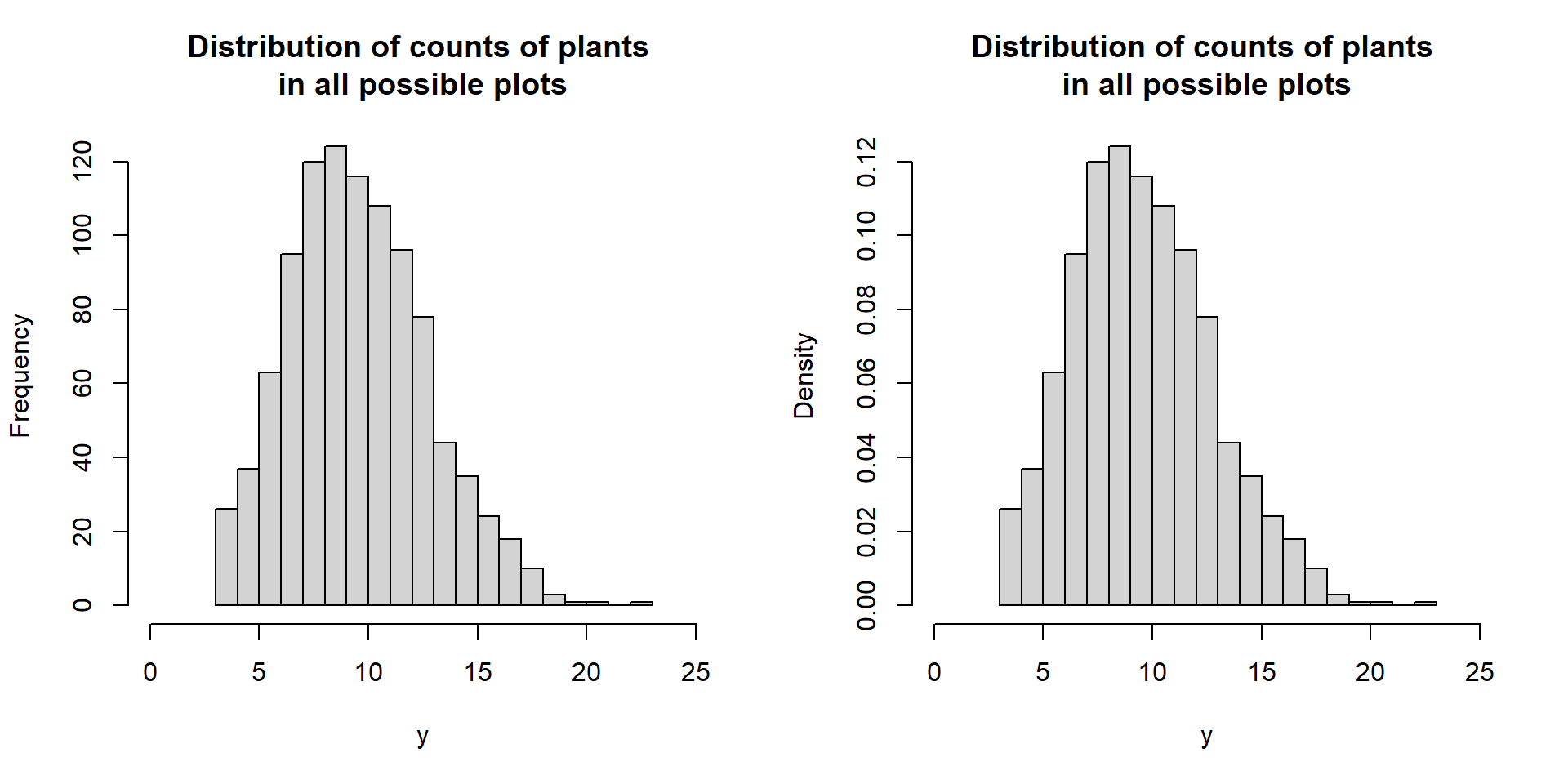
Toss of a coin
Roll of a die
Weight of a captured elk
Count of plants in a sampled plot


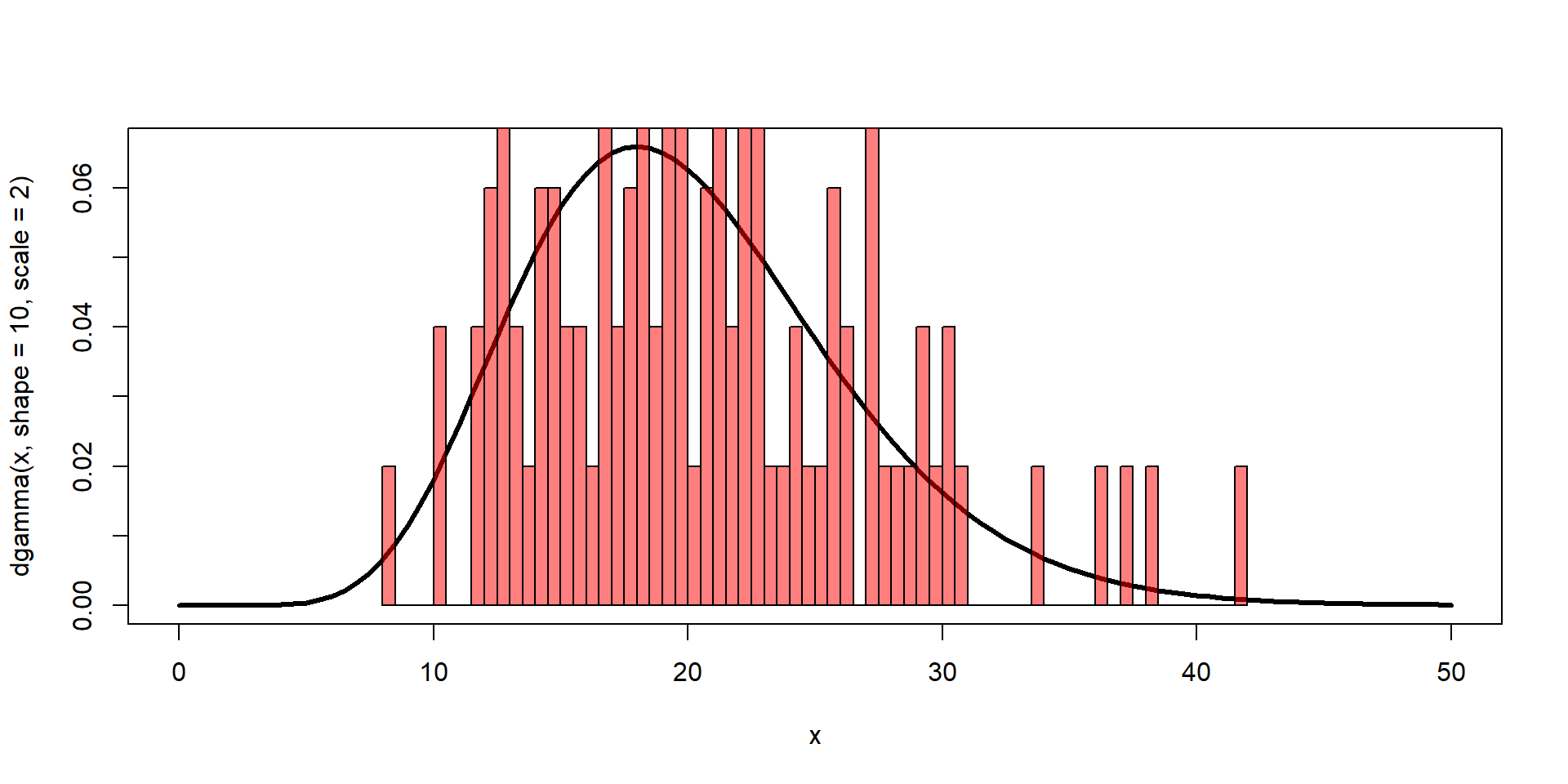
The values observed can be understand based on the frequency within the population or presumed super-population. These frequencies can be described by probabilities.

Frequency / Probabilitities

par(mfrow=c(1,2))
hist(y, breaks=20,xlim=c(0,25),main=main)
hist(y, breaks=20,xlim=c(0,25),freq = FALSE,main=main)

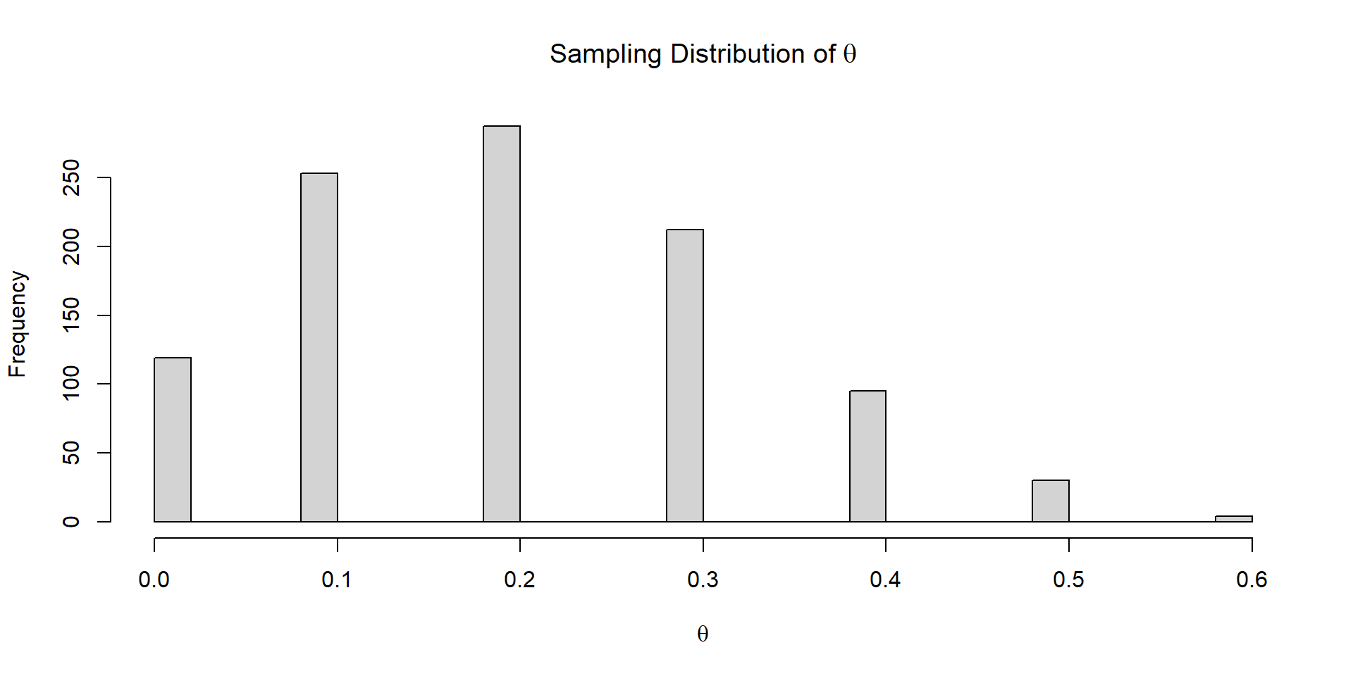
We often only get to see ONE sample from this distribution.

Random Variables

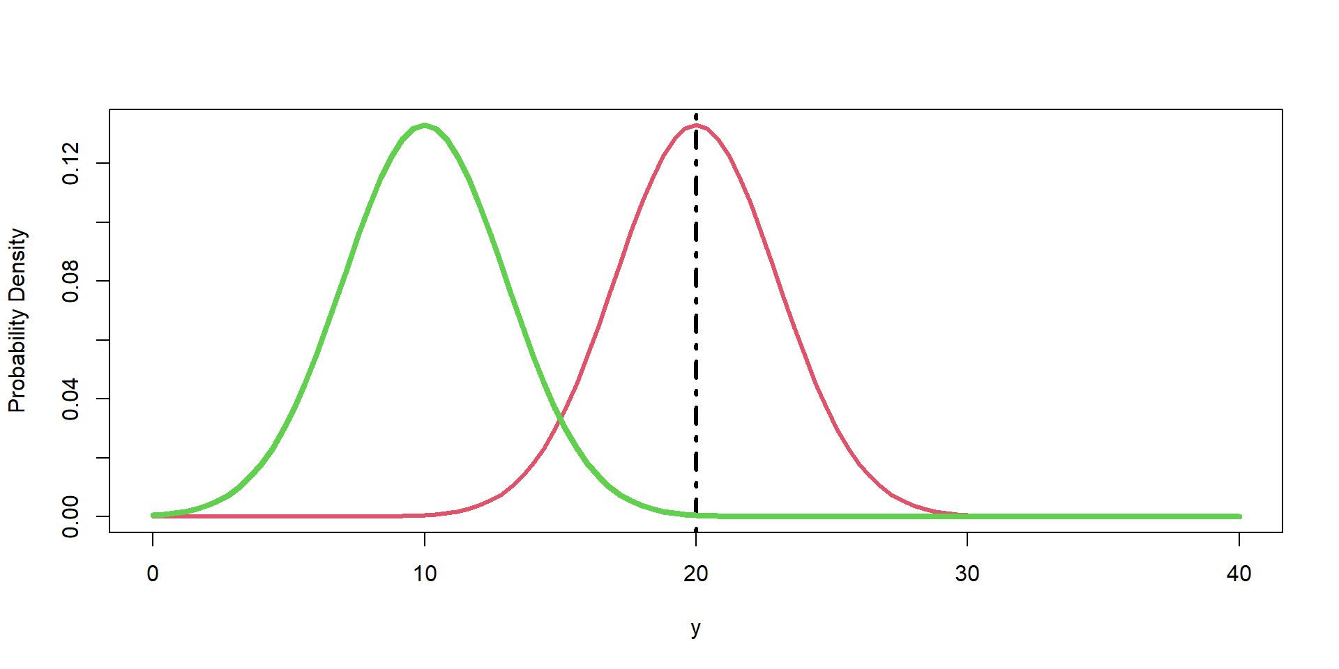
We are often interested in the characteristics of the whole population of frequencies,

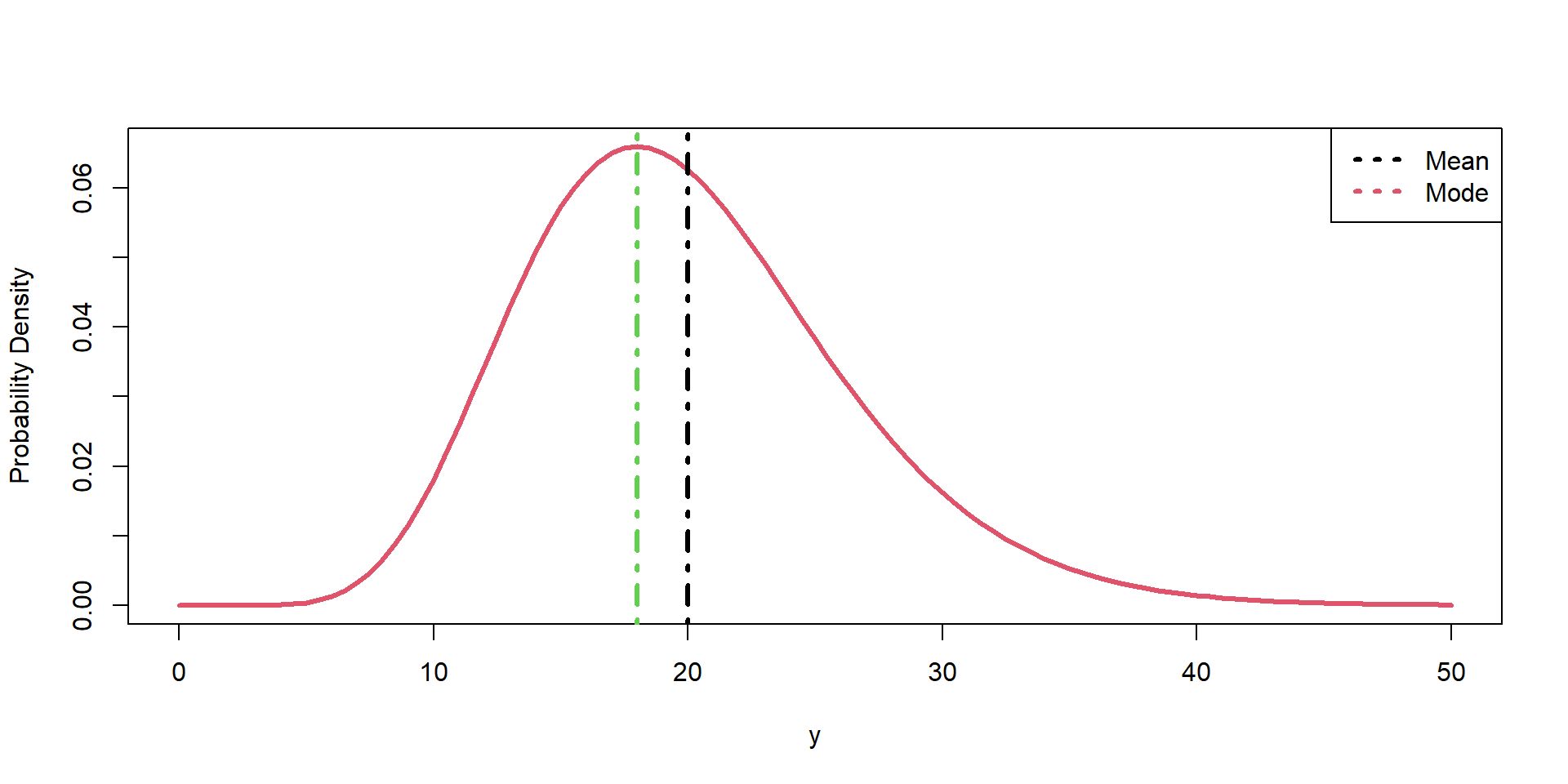
  • central tendency (mean, mode, median)
  • variability (var, sd)
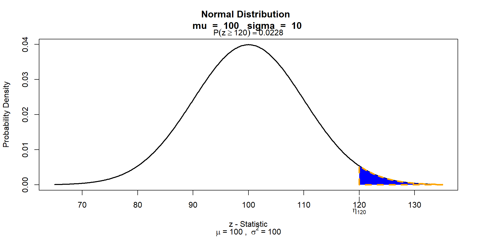
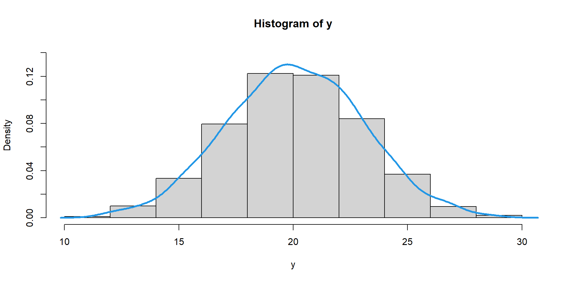
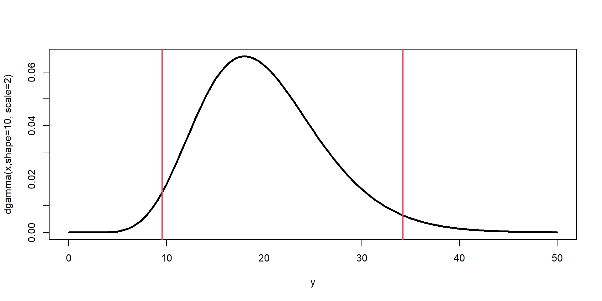
  • proportion of the population that meets some condition
    P(\(8 \leq y \leq\) 12) =0.68

We infer what these are based on our sample (i.e., statistical inference).

Philosophy

Frequentist Paradigm:

Data (e.g., \(y\)) are random variables that can be described by probability distributions with unknown parameters that (e.g., \(\theta\)) are fixed (scalars).


Bayesian Paradigm:

Data (e.g., \(y\)) are random variables that can be described by probability functions where the unknown parameters (e.g., \(\theta\)) are also random variables that have probability functions that describe them.

Random Variables

\[ \begin{align*} y =& \text{ event/outcome} \\ f(y|\boldsymbol{\theta}) =& [y|\boldsymbol{\theta}]= \text{ process governing the value of } y \\ \boldsymbol{\theta} =& \text{ parameters} \\ \end{align*} \]

\(f()\) or [ ] is conveying a function (math).

It is called a PDF when \(y\) is continuous and a PMF when \(y\) is discrete.

  • PDF: probability density function
  • PMF: probability mass function

Functions

We commonly use deterministic functions (indicated by non-italic letter); e.g., log(), exp(). Output is always the same with the same input. \[ \hspace{-12pt}\text{g} \\ x \Longrightarrow\fbox{DO STUFF } \Longrightarrow \text{g}(x) \]

\[ \hspace{-14pt}\text{g} \\ x \Longrightarrow\fbox{+7 } \Longrightarrow \text{g}(x) \]

\[ \text{g}(x) = x + 7 \]

Random Variables

Probability: Interested in \(y\), the data, and the probability function that “generates” the data. \[ \begin{align*} y \leftarrow& f(y|\boldsymbol{\theta}) \\ \end{align*} \]

Statistics: Interested in population characteristics of \(y\); i.e., the parameters,

\[ \begin{align*} y \rightarrow& f(y|\boldsymbol{\theta}) \\ \end{align*} \]

Probability Functions

Special functions with rules to guarantee our logic of probabilities are maintained.

Discrete RVs

\(y\) can only be a certain set of values.

  1. \(y \in \{0,1\}\)
    • 0 = dead, 1 = alive
  2. \(y \in \{0,1, 2\}\)
    • 0 = site unoccupied, 1 = site occupied w/o young, 2 = site occupied with young
  3. \(y \in \{0, 1, 2, ..., 15\}\)
    • count of pups in a litter; max could by physiological constraint

These sets are called the sample space (\(\Omega\)) or the support of the RV.

PMF

\[ f(y) = P(Y=y) \]

Data has two outcomes (0 = dead, 1 = alive)

\(y \in \{0,1\}\)

There are two probabilities

  • \(f(0) = P(Y=0)\)
  • \(f(1) = P(Y=1)\)

Axiom 1: The probability of an event is greater than or equal to zero and less than or equal to 1.

\[ 0 \leq f(y) \leq 1 \] Example,

  • \(f(0) = 0.1\)
  • \(f(1) = 0.9\)

Axiom 2: The sum of the probabilities of all possible values (sample space) is one.

\[ \sum_{i} f(y_i) = f(y_1) + f(y_2) + ... = P(\Omega) =1 \] Example,

  • \(f(0) + f(1) = 0.1 + 0.9 = 1\)

PMF

Still need to define \(f()\), our PMF for \(y \in \{0,1\}\)

The Bernoulli distribution

\[ f(y|\theta) = [y|\theta]= \begin{align} \theta^{y}\times(1-\theta)^{1-y} \end{align} \]

\(\theta\) = P(Y = 1) = 0.2

\[ f(y|\theta) = [y|\theta]= \begin{align} = 0.2^{1}\times(1-0.2)^{0-0} \end{align} \]

\[ f(y|\theta) = [y|\theta]= \begin{align} = 0.2 \times (0.8)^{0} = 0.2 \end{align} \]

Bernoulli PMF

\[ f(y|\theta) = [y|\theta]= \begin{align} \theta^{y}\times(1-\theta)^{1-y} \end{align} \]

Sample space support (\(\Omega\)):

  • \(y \in \{0,1\}\)

Parameter space support (\(\Theta\)):

  • \(\theta \in [0,1]\)
  • General: \(\theta \in \Theta\)

Bernoulli PMF (Code)

What would our data look like for 10 ducks that had a probability of survival (Y=1) of 0.20?

#Define inputs
  theta=0.2;  N=1 

#Random sample - 1 duck
  rbinom(n=1,size=N,theta)
[1] 0
#Random sample - 10 ducks
  rbinom(n=10,size=N,theta)
 [1] 1 0 0 0 1 0 1 0 1 0

Why is this useful to us?

How about to evaluate the sample size of ducks needed to estimate \(\theta\)?

y.mat = replicate(1000,rbinom(n = 10,size=N,theta))
theta.hat = apply(y.mat, 2, mean)

Binomial PMF

The Bernoulli is a special case of the Binomial Distribution.

\[ f(y|\theta) = [y|\theta]= \begin{align} {N\choose y} \theta^{y}\times(1-\theta)^{N-y} \end{align} \]

\(N\) = total trials / tagged and released animals


\(y\) = number of successes / number of alive animals at the of the study.

Binomial PMF (Code)

# 1 duck tagged/released and one simulation
  theta=0.2;  N=1 
  rbinom(n=1,size=N,theta)
[1] 1
# 1000 ducks tagged/released and one simulation
  theta=0.2;  N=1000 
  rbinom(n=1,size=N,theta)
[1] 198
# 1000 ducks tagged/released and 10 simulation
  theta=0.2;  N=1000 
  rbinom(n=10,size=N,theta)
 [1] 180 190 198 192 169 192 192 217 206 216
# 1 duck tagged for each of 1000 simulations
  theta=0.2;  N=1
  y = rbinom(n=1000,size=N,theta)
  y
   [1] 0 0 0 1 0 0 0 0 0 1 0 0 0 0 0 0 0 0 1 0 0 0 0 1 0 0 0 1 0 0 0 0 0 0 0 1 0
  [38] 0 0 0 1 0 0 0 1 0 1 0 0 0 0 0 0 0 0 0 0 1 0 0 0 0 0 0 0 0 0 0 0 1 0 0 1 0
  [75] 0 0 0 0 0 0 0 0 0 0 0 0 0 0 1 0 1 1 0 0 0 1 0 0 0 0 0 0 0 0 0 0 0 0 0 0 0
 [112] 1 1 0 0 0 0 1 0 0 0 0 0 0 0 1 1 0 0 0 0 0 0 0 0 0 0 1 0 0 0 1 1 0 0 1 0 0
 [149] 0 0 0 0 1 0 0 0 0 1 0 0 0 0 0 0 0 0 0 0 0 0 0 1 0 0 0 0 1 0 0 0 0 0 0 0 0
 [186] 1 0 0 1 0 1 0 0 1 0 0 0 0 0 1 0 0 0 0 0 0 0 0 0 1 0 0 0 0 0 0 0 1 0 0 0 0
 [223] 0 0 0 0 0 1 0 0 1 0 0 0 0 0 0 0 1 0 0 0 0 0 0 0 1 0 0 0 1 1 1 0 0 0 1 0 0
 [260] 0 1 1 0 0 1 0 0 0 1 0 1 1 1 0 0 0 0 0 0 0 0 0 0 0 0 0 0 0 0 0 0 1 0 0 0 0
 [297] 0 1 0 0 0 0 0 0 0 0 1 0 0 0 0 0 0 1 1 0 0 0 0 0 1 0 0 0 0 0 0 0 0 1 0 0 0
 [334] 0 1 0 0 0 1 0 0 0 0 0 0 0 0 0 0 0 0 0 0 0 0 0 0 1 0 0 0 0 0 0 0 0 0 0 0 0
 [371] 0 0 0 1 0 0 0 0 0 0 1 0 0 0 0 1 0 0 0 0 1 0 0 0 1 0 0 1 0 0 0 0 0 1 0 0 1
 [408] 0 0 0 0 0 1 0 0 0 0 0 1 0 0 0 1 0 0 0 1 0 0 0 0 0 0 1 0 0 0 0 0 0 0 0 1 0
 [445] 0 0 0 0 0 0 0 0 0 0 0 1 0 0 0 0 0 1 0 0 0 0 1 0 0 0 1 0 0 0 0 0 1 0 0 0 0
 [482] 0 0 1 0 0 0 0 0 0 0 0 0 0 1 0 0 0 0 1 0 1 0 0 0 0 0 0 0 0 0 0 0 0 0 0 0 1
 [519] 0 0 1 1 0 0 0 1 0 0 0 0 0 0 1 1 0 0 0 1 0 0 1 0 1 0 0 1 1 0 0 0 1 0 1 0 0
 [556] 1 0 0 0 1 1 0 0 0 0 1 1 1 0 0 0 0 0 0 0 0 0 0 0 0 1 0 0 0 0 0 1 0 0 1 0 0
 [593] 1 0 0 0 0 0 0 1 1 0 1 0 0 1 1 0 0 0 0 0 0 1 0 0 1 0 0 0 1 0 0 1 0 0 0 0 0
 [630] 0 1 0 1 0 0 0 0 0 0 0 0 0 0 1 1 1 0 0 0 0 0 0 0 0 0 1 1 1 1 0 0 0 0 1 0 1
 [667] 0 1 0 0 0 1 0 0 0 0 0 0 0 0 0 0 1 1 0 0 0 0 0 0 0 0 0 1 0 0 0 1 0 1 0 0 0
 [704] 0 1 0 0 0 0 0 1 1 0 0 0 0 0 0 0 0 0 0 0 0 0 0 0 0 0 0 0 0 0 0 1 0 0 0 0 0
 [741] 0 0 0 0 0 0 1 0 0 0 0 0 0 0 0 0 0 0 0 0 0 0 0 0 1 0 0 0 0 0 0 0 0 0 0 0 1
 [778] 0 0 0 0 0 0 0 0 1 0 0 0 0 0 0 0 0 0 0 1 0 0 0 0 0 0 0 0 1 1 0 0 0 0 0 0 1
 [815] 0 1 0 0 0 1 1 0 1 0 0 0 0 0 0 1 1 0 1 0 0 1 0 0 1 0 0 0 0 1 1 0 0 0 0 0 0
 [852] 1 0 0 0 0 1 0 0 0 0 0 0 1 1 0 0 0 0 0 0 0 1 0 0 1 0 0 0 0 0 0 0 1 0 0 0 0
 [889] 0 0 1 0 0 0 0 1 0 0 0 1 0 0 0 0 0 0 0 0 1 0 0 0 1 0 1 1 0 0 0 1 1 0 0 0 0
 [926] 0 0 1 0 1 0 0 0 0 0 0 0 0 0 0 1 0 0 0 1 1 0 1 0 0 0 0 0 0 1 0 0 0 0 0 0 0
 [963] 0 1 0 0 0 0 0 0 0 0 0 0 0 0 1 0 1 0 0 0 1 0 0 0 0 0 0 0 1 1 0 0 0 0 0 0 0
[1000] 0
sum(y)
[1] 186

Support

Use a probability function that makes sense for your data/RV. In Bayesian infernece, we also pick prob. functions that make sense for parameters.


The sample space and parameter support can be found on Wikipedia for many probability functions.

Normal PDF

For example, the Normal/Gaussian distribution describes the sample space for all values on the real number line.

\[y \sim \text{Normal}(\mu, \sigma) \\ y \in (-\infty, \infty) \\ y \in \mathbb{R}\]

What is the parameter space for \(\mu\) and \(\sigma\)?

Normal Distribution

We collect data on adult alligator lengths (in).

 [1]  90.30  83.02 103.67  85.17  99.20 106.74  90.76 105.28  99.41 101.72


Should we use the Normal Distribution
to estimate the mean?

Does the support of our data match
the support of the PDF?

What PDF does?

Are they exactly the same?


The issue is when the data are near 0, we might estimate non-sensical values (e.g. negative).

PDF

Continuous RVs

\(y\) are an uncountable set of values.


Provide ecological data examples that match the support?

  1. Gamma: \(y \in (0,\infty)\)
  2. Beta: \(y \in (0,1)\)
  3. Continuous Uniform: \(y \in [a,b]\)

PDF

PDFs of continious RVs follow the same rules as PMFs.

Confusing Differences

Axiom 1:

  • \(f(y) \geq 0\)

PDFs output probability densities, not probabilities.


Axiom 2:

  • Probs are the area b/w a lower and upper value of \(y\); i.e, area under the curve

\[ y \sim \text{Normal}(\mu, \sigma) \\ f(y|\mu,\sigma ) = \frac{1}{\sigma\sqrt{2\pi}}e^{\frac{1}{2}(\frac{y-\mu}{\sigma})^{2}} \\ \]

visualize.it(dist = 'norm', stat = c(100),
             list(mu = 100 , sd = 10), section = "upper")

The math,

\[ \int_{120}^{\infty} f(y| \mu, \sigma)dy = P(120<Y<\infty) \]

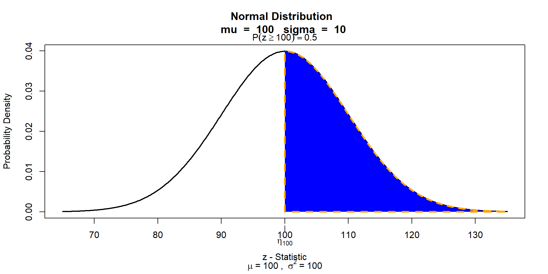
Read this as “the integral of the probability density function between 120 and infinity (on the left-hand side) is equal to the probability that the outcome of the random variable is between 120 and infinity (on the right-hand side)”.


The code

pnorm(120,mean=100,sd=10,lower.tail = FALSE)
[1] 0.02275013


Or, we could reverse the question.

qnorm(0.02275,100,10,lower.tail = FALSE)
[1] 120

PDF

Axiom 3:

  • \(\int_{\text{lower support}}^{\text{upper suppport}}f(y)dy = 1\)

The sum of the probability densities of all possible outcomes is equal to 1.

Normal Distribution (PDF Code)

y = rnorm(1000, mean = 20, sd = 3)
hist(y,freq=FALSE,ylim=c(0,0.14))
lines(density(y),lwd=3,col=4)

Normal Distribution (PDF Code)

curve(dnorm(x, mean= 20, sd = 3),
      xlim=c(0,40),lwd=3,col=2,ylab="Probability Density",xlab="y")
abline(v=20, lwd=3, col=1, lty=4)

Normal Distribution (PDF Code)

curve(dnorm(x, mean = 10, sd = 3),xlim=c(0,40),lwd=4,col=3,add=TRUE)

Moments

Properties of all probability functions.

  • 1\({^{st}}\) moment is central tendency
  • 2\({^{nd}}\) moment is the dispersion

Normal Distribution: parameters (\(\mu\) and \(\sigma\)) are 1\({^{st}}\) and 2\({^{nd}}\) moments

Moments

Gamma Distribution: parameters are not moments

Parameters

Shape = \(\alpha\), Rate = \(\beta\)

OR

Shape = \(\kappa\), Scale = \(\theta\), where \(\theta = \frac{1}{\beta}\)

NOTE: probability functions can have Alternative Parameterizations, such they have different parameters.

Moments are functions of these parameters:

  • mean = \(\kappa\theta\) or \(\frac{\alpha}{\beta}\)

  • var = \(\kappa\theta^2\) or \(\frac{\alpha}{\beta^2}\)

Gamma Distribution

Probability: Interested in the variation of y, \[ \begin{align*} y \leftarrow& f(y|\boldsymbol{\theta'}) \\ \end{align*} \]

\[ \begin{align*} \boldsymbol{\theta'} =& \begin{matrix} [\kappa & \theta] \end{matrix} \\ f(y|\boldsymbol{\theta}') &= \text{Gamma(}\kappa, \theta) \\ \end{align*} \]

\[ \begin{align*} f(y|\boldsymbol{\theta}') &= \frac{1}{\Gamma(\kappa)\theta^{\kappa}}y^{\kappa-1} e^{-y/\theta} \\ \end{align*} \]

Sample/parameter Support:

  • \(y \in (0,\infty)\)
  • \(\kappa \in (0,\infty)\)
  • \(\theta \in (0,\infty)\)

Gamma Distribution (PDF Code)

Gamma Wikipedia

shape =10
scale = 2

mean1 = shape*scale
mean1
[1] 20
mode1 = (shape-1)*scale
mode1
[1] 18
stdev = sqrt(shape*scale^2)
stdev
[1] 6.324555

Gamma Distribution (PDF Code)

Gamma Distribution

What is the probability we would sample a value >40?
In this population, how common is a value >40?

\[ \begin{align*} p(y>40) = \int_{40}^{\infty} f(y|\boldsymbol{\theta}) \,dy \end{align*} \]

pgamma(q=40, shape=10, scale=2,lower.tail=FALSE)
[1] 0.004995412


What is the probability of observing \(y\) < 20

pgamma(q=20,shape=10, scale=2,lower.tail=TRUE)
[1] 0.5420703


What is the probability of observing 20 < \(y\) < 40

pgamma(q=40,shape=10, scale=2,lower.tail=TRUE)-
pgamma(q=20,shape=10, scale=2,lower.tail=TRUE)
[1] 0.4529343


Reverse the question: What values of \(y\) and lower have a probability of 0.025

qgamma(p=0.025,shape=10, scale=2,lower.tail=TRUE)
[1] 9.590777


What values of \(y\) and higher have a probability of 0.025

qgamma(p=0.025,shape=10, scale=2,lower.tail=FALSE)
[1] 34.16961
curve(dgamma(x,shape=10, scale=2),xlim=c(0,50),lwd=3,
      xlab="y", ylab="dgamma(x,shape=10, scale=2)")
abline(v=c(9.590777,34.16961),lwd=3,col=2)

We can consider samples from this population,

set.seed(154434)
y <- rgamma(100, shape=10, scale=2)

The others side of the coin

Statistics: Interested in estimating population-level characteristics; i.e., the parameters

\[ \begin{align*} y \rightarrow& f(y|\boldsymbol{\theta}) \\ \end{align*} \]

REMEMBER

\(f(y|\boldsymbol{\theta})\) is a probability statement about \(y\), NOT \(\boldsymbol{\theta}\).