Big Picture
Science and Modeling

What’s the point of statistics?

a process of learning through empirical observations

together, science philosophy and statistical modeling is the backbone to empirical learning

Today

1. Study Objectives, Hypotheses, and Predictions

2. Big Data and Sampling

3. Inference and Prediction

4. Model-Based vs Design-Based Sampling/Inference

Lab: Simulation and Markdown

Study Objective

Definition

What you want to accomplish; can have multiple related objectives in a single manuscript.

Example

To understand the space-use of coyotes.

Framing the importance of the objective(s) provides the justification and depends on the audience.

Hypothesis

Definition

A story that explains how the world works
An explanation for an observed phenomenon

Example (weak)

Coyotes have small home ranges in urban areas

Research/Scientific Hypothesis

Definition

“A statement about a phenomenon that also includes the potential mechanism or cause of that phenomenon”. (Betts et al. 2021)

Example

Coyotes have small home ranges in urban areas because food resource density is high

Non-hypothesis hypothesis: We hypothesize variation in coyote home range size.

Statistical Model/Hypothesis

Definition

An explicit mathematical and stochastic representation of the observational & mechanistic process of the empirical observations.

Statistical Model/Hypothesis

Example:

\[\textbf{y} = \beta_0 + \beta_1 \times \textbf{x} + \mathbf{\epsilon}\] \[\mathbf{\epsilon} \sim \text{Normal}(0, \sigma^2)\]

where…

\(\textbf{y}\) = vector of home range sizes of coyotes
\(\beta_0\) = intercept
\(\beta_1\) = effect diff. of HR size for urban coyotes
\(\textbf{x}\) = indicator of HR in urban (1) or not in urban (0)
\(\sigma^2\) = uncertainty / unknown variability

Statistical Model/Hypothesis

Example:

\[\textbf{y} = \beta_0 + \beta_1 \times \textbf{x} + \mathbf{\epsilon}\] \[\mathbf{\epsilon} \sim \text{Normal}(0, \sigma^2)\]

Evidence of hypothesis support

\(\beta_1\) is negative and statistically clearly different¹ than zero

Prediction

Definition

The expected outcome from a hypothesis. If agrees with data, it would support the hypothesis or at least not reject it.

Example 1

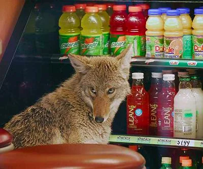
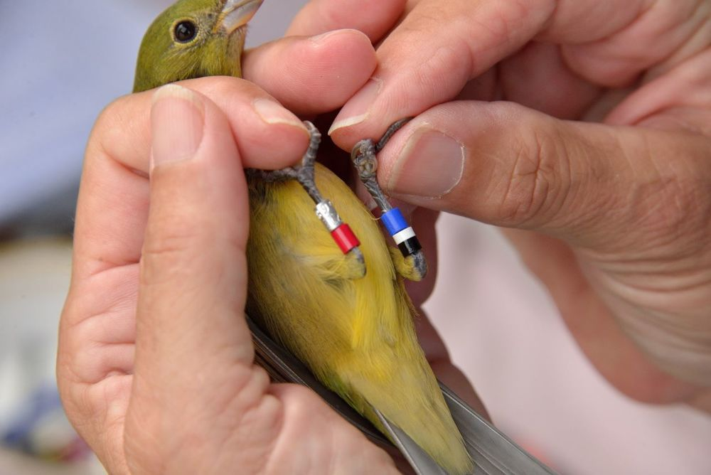
Okay: Coyote home ranges are smaller in urban areas compared to non-urban areas

Example 2

Better: Coyote home ranges in urban areas with high available food resources is smaller than coyote home ranges in urban areas with less available food resources and smaller than coyotes living in non-urban areas

Types of Studies

Descriptive/Naturalist (not hypothetico-deductive)
Hypothetico-Deductive Observational
Hypothetico-Deductive Experimental

Manuscript Writing

Where do you put these?

objectives
justification of objectives
hypotheses
predictions

Take-Aways?

1. Study Objectives, Hypotheses, and Predictions

Data is everywhere
It is the era of BIG DATA!

Big Data Problems

“The hidden Biases of Big Data” by Kate Crawford in Harvard Business Review (2013)

“with enough data, the numbers speak for themselves”- Wired Magazine Editor

Big Data Problems

“The hidden Biases of Big Data” by Kate Crawford in Harvard Business Review (2013)

"Data and data sets are not objective;"

"they are creations of human design."

Big Data Problems

The Annals of Applied Statistics (2018); Xiao Li Meng,

The Big Data Paradox:

"the bigger the data, the surer we fool ourselves” ... when we fail to account for our sampling process.

Sampling Processes == Human Design

Big Data Problems

Bradley et al. 2021 (Nature)

"...data quality matters more than data quantity, and that compensating the former with the latter is a mathematically provable losing proposition."

Big Data Problems

Using eBird data w/o accounting for sampling biases.

Link1. Link2.

The Questioning Scientist

In regard to data and statistical models, 21^st century scientists should be pragmatic, excited, and questioning.

How and why did these data come to be?
- understand how the data came to be
- ask this even when you design the study, after data collection

What do these data look like?
- visualize the data in many dimensions
- keep in mind - not all outcomes are visible in data – example?

How does this statistical model work?
- statistical notation, explicit and implicit assumptions, optimization

How does this statistical model fail in theory and in practice?
- statistical robustness and identifiability

Data vs. Information

Data = Numbers/Groupings

Data ≠ Information

Information

Data contains information, depending on ...

the question being asked of the data
how the data came to be
the goal of the question

The question and the data

Ecological surveillance monitoring will often have low quality information regarding post-hoc hypotheses.

Example?

The goal of the question

learn about the data (data summary)
apply learning outside of the data (inference)
learn about conditions relevant to but not observed in the data (prediction)

inference and prediction are different goals, optimally requiring different data, statistical modeling proecdures.

BUT, are also not mutually exclusive.

Take-Aways

1. Study Objectives, Hypotheses, and Predictions

2. Big Data and Sampling

Inference and Prediction

Which is worse?

unbiased imprecise result
precise biased result

Inference and Prediction

From "The strategy of model building in population biology" by Richard Levins (American Scientists, 1966) :

"It is of course desirable to work with manageable models which maximize generality, realism, and precision toward the overlapping but not identical goals of understanding, predicting, and modifying nature. But this cannot be done."

Inference and Prediction

From "To Explain or to Predict" by Galit Shmueli (Statistical Science, 2010):

Explanatory modeling focuses on minimizing (statistical) bias to obtain the most accurate representation of the underlying theory.

Predictive modeling focuses on minimizing both bias and estimation variance; this may sacrifice theoretical accuracy for improved empirical precision.

Inference and Prediction

This leads to a strange result:

the "wrong" statistical model can predict better than the correct one.

BUT …

Explanatory models will likely perform better when predicting outside of the sample space and the model has the core underlying processes

Inference and Prediction

Trade-Off between prediction accuracy and model interpretability; from James et al. 2013. An Introduction to Statistical Learning

Design- and Model-Based Sampling/Inference

Take-Aways

1. Study Objectives, Hypotheses, and Predictions

2. Big Data and Sampling

3. Inference and Prediction

When do we need statistics?

Design-Based

Thompson, 2012. Sampling.

The sample and population are what??

Design-Based

inference relies on randomly assigning some units to be in the sample (e.g., random sampling).

Design-Based

the values themselves are held to be fixed, whereas the sampling process is random.

Design-Based

Key Strengths: the population of interest is often defined (e.g., grid area); does not relying on stochastic models representing the structure of the data for reliable inference

Key Weaknesses: limited in application; still requires models to accommodate observational processes, such as detection probability

Design-Based

\(\textbf{Y}\) = [\(y_1\),…,\(y_N\)]

This means something different:

\(\textbf{Y}\) = (\(y_1\),…,\(y_N\))

(stuff) is exclusive of end points
[stuff] is inclusive of end points

Design-Based

\(\textbf{Y}\) = [\(y_1\),…,\(y_N\)]
The mean is \(\bar{Y} = \sum_{i=1}^N Y_i / N\) and the sample mean is \(\hat{\bar{y}} = \sum_{i=1}^n y_i / n\)

The population mean describes ….?

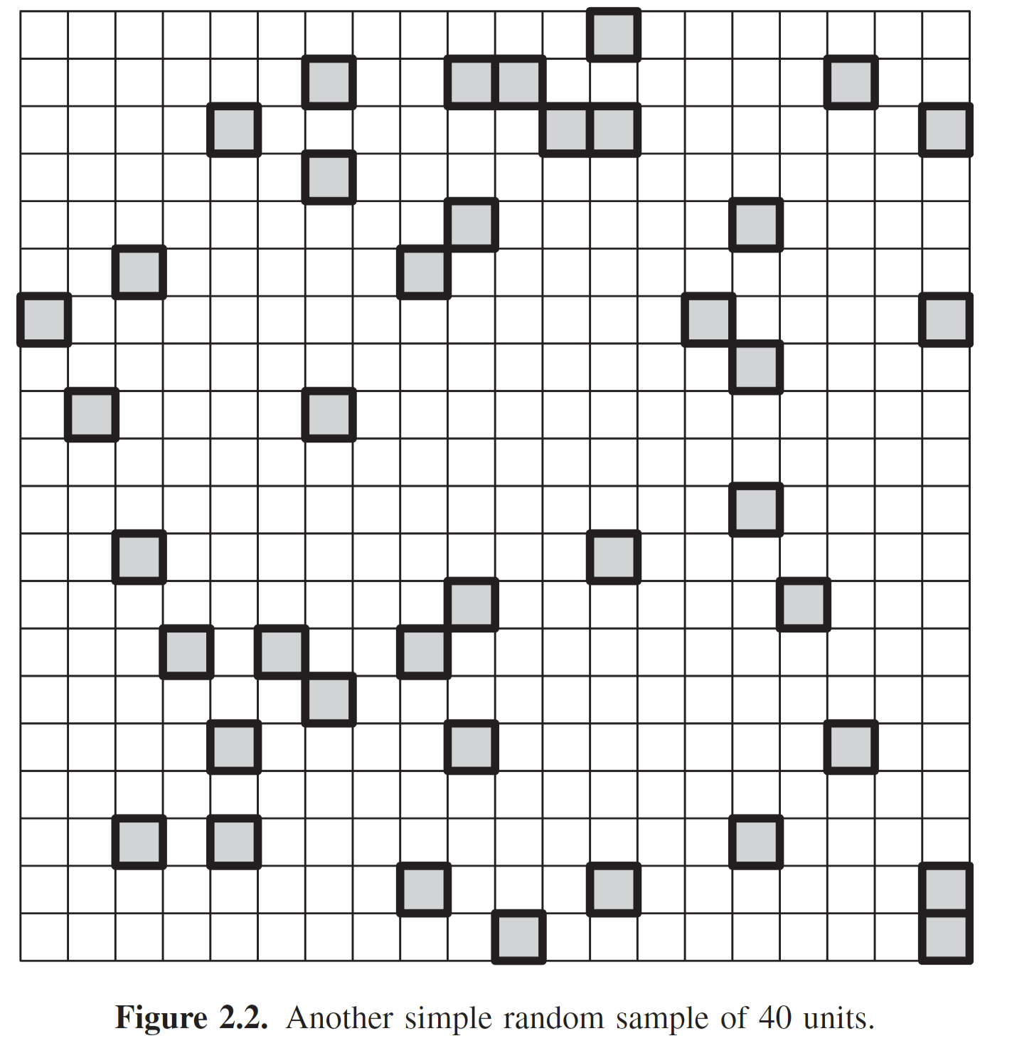
\(\textbf{y}\) is a random vector that has \(n\) random variables. One sample of 4 cells.

\(\boldsymbol{y} = \begin{matrix} [y_{1} & y_{2} & y_{3} & y_{4 }]\end{matrix}\)

\(\boldsymbol{y}' = \boldsymbol{y}^{T} = \begin{bmatrix} y_{1} & \\y_{2} &\\ y_{3} & \\y_{4 }\end{bmatrix}\)

Random Variable

Wikipedia: A random variable (also called ‘random quantity’ or ‘stochastic variable’) is a mathematical formalization of a quantity or object which depends on random events.

We observe samples from the domain or population or sampling frame.

Samples are observed with some probability.

Statistic

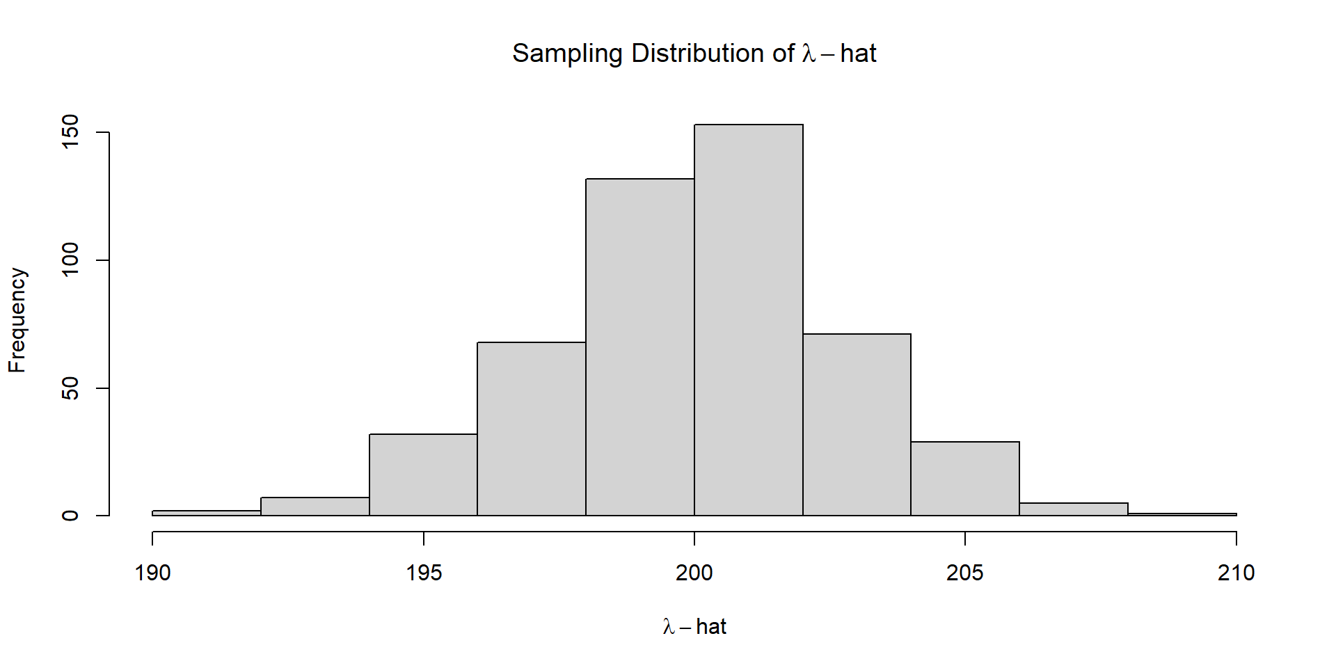
\(\hat{\bar{y}}\) is a ‘statistic’ (# computed from a sample) and is also a random variable

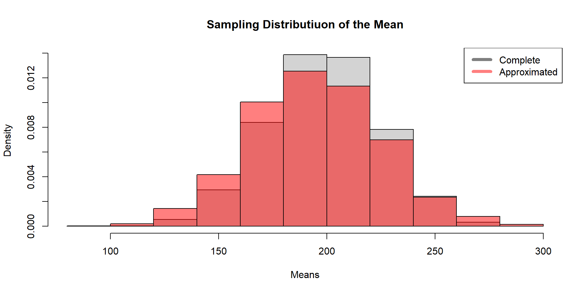
statistics have a sampling distribution, describing the probability associated to observing different values of the statistic

Design-Based Code

TRUTH

#random discrete uniform sampler
rdu<-function(n,lower,upper){sample(lower:upper,n,replace=T)}

mat = matrix(rdu(25, 
                 lower = 0, 
                 upper = 400
                 ),
             nrow=5, ncol=5
             )
mat

     [,1] [,2] [,3] [,4] [,5]
[1,]   51   33  294  191  366
[2,]  184   71  312  302  290
[3,]   99  285   98  336  128
[4,]    0  298  105   15  294
[5,]  216  224   88  341   30

Design-Based Code

Random Sampling

  n = 10
  y = sample(
             c(mat),
             10, 
             replace = TRUE
             )
  y

 [1] 216 285 216  30 312 341 216  71  30 294

Estimator for the population mean

  mean(y)

[1] 201.1

Design-Based Code

Sampling Distribution

# How many ways can we uniquely sample 10 things from 25
combs = function(n, x) {
  factorial(n) / factorial(n-x) / factorial(x)
}

combs(25, 10)

[1] 3268760

Design-Based Code

Get Every combination and then calcualte the mean for each sample of 10

  set.seed(5435)
  all.combs = utils::combn(c(mat), 10)
  dim(all.combs)

[1]      10 3268760

  mean.all.combs = apply(all.combs,2,mean)

Design-Based Code

OR, we can sample enough times to approximate it

  set.seed(5435)
  sim.sampling.dist=replicate(2000,
                              sample(c(mat),10)
                              )
  dim(sim.sampling.dist)

[1]   10 2000

  mean.samples = apply(sim.sampling.dist,2,mean)

Design-Based Code

Model-Based

Inference relies on …

“a statistical model describing how observations on population units are thought to have been generated from a super‐population with potentially infinitely many observations for each unit;” Williams and Brown, 2019

“The analysis need not account for sampling randomization, because the sample is considered fixed. However, the unit values are considered random.” Williams and Brown, 2019

Model-Based

BUT….

when linking ‘unit values’ in a model, we need to account for their dependence.

Randomization allows us to make conditional independence claims among data in our sample, thus the model is simpler.

\(P(y_{2}|y_{1}) = P(y_{2})\)

Model-Based

Key Strengths: Very flexible. Modeling is magic.

Key Weaknesses: 1) Can be difficult to assess assumptions and 2) sampling frame is not always clear and thus the population you are infering to is not entirely clear

Model-Based

\(\textbf{y} \sim\) Poisson(\(\lambda\)) Wikipedia link
\(y_{i} \sim\) Poisson(\(\lambda\))

\(\lambda\) is the population mean and variance

Sample mean Estimator \(\hat{\lambda} = \sum_{i=1}^n y_{i}/n\)

Maximum-Likelihood Estimate (MLE)

Model-Based Code

#Create a function, to be replicated
  lambda=200
  n.sim=500
  mat.fn = function(lambda){matrix(rpois(25, lambda=lambda),
                               nrow=5, ncol=5
                               )
  }

Model-Based Code

# repeat the function n.sim times
  list.mat = replicate(n.sim, 
                       mat.fn(lambda), 
                       simplify=FALSE
                       )
  length(list.mat)

[1] 500

#One realization
  list.mat[[1]]

     [,1] [,2] [,3] [,4] [,5]
[1,]  213  221  202  204  173
[2,]  195  182  193  190  215
[3,]  221  216  187  182  179
[4,]  176  196  218  210  211
[5,]  218  182  193  229  188

# Sample mean for the first realization
  mean(list.mat[[1]])

[1] 199.76

Model-Based Code

Sampling Distribution

lambda.hat = unlist(lapply(list.mat,FUN=mean))

Statistical Bias

the difference b/w the true value and the mean of the sampling distribution of all possible values; applies to design- and model-based sampling

Statistical Bias (Code)

# Bias
  mean(lambda.hat) - lambda

[1] 0.00544

# relative bias
  (mean(lambda.hat) - lambda)/lambda

[1] 2.72e-05

Precision of the mean (Code)

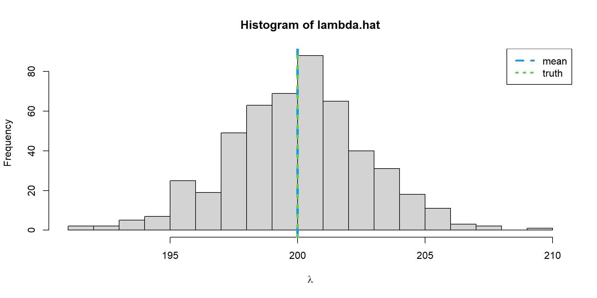
What is the probability that we will observe a mean within 5% of the truth?

We can calculate this using Monte Carlo integration

  diff = 0.025*lambda
  diff

[1] 5

  lower = lambda-diff
  upper = lambda+diff

  index = which(lambda.hat>=lower & lambda.hat <= upper)

#Probability of getting a mean within 5% of the truth
  length(index)/n.sim

[1] 0.934

Take-Aways

1. Study Objectives, Hypotheses, and Predictions

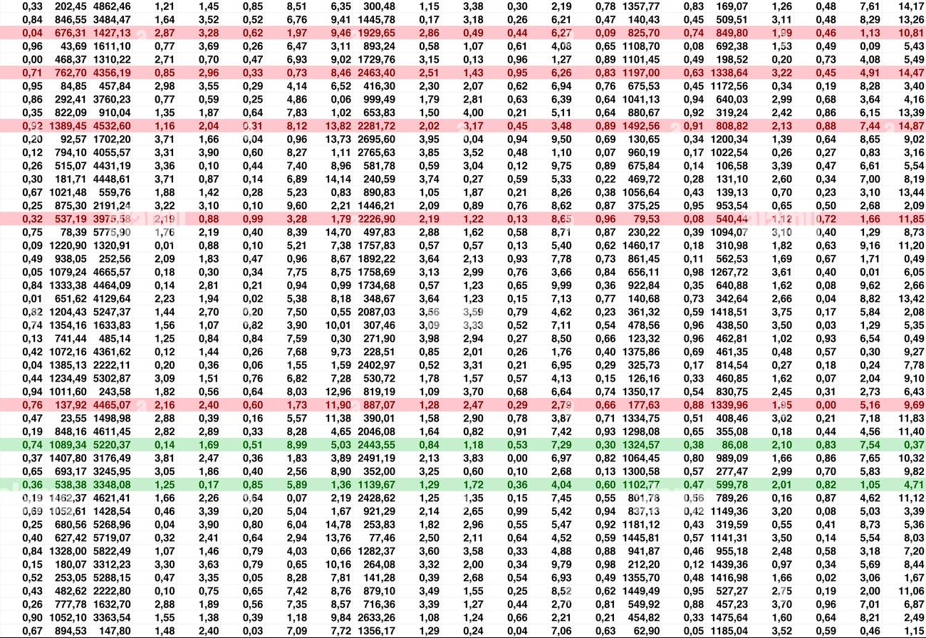
2. Big Data and Sampling

3. Inference and Prediction

4. Model-Based vs Design-Based Inference

Lab

Objectives

Introduce R Markdown
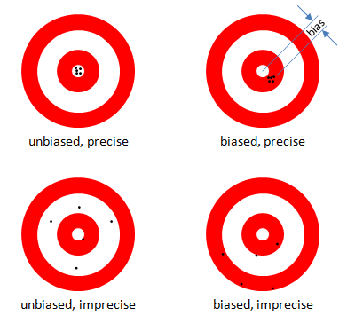
Use simulation and design-based sampling to investigate bias and precision

Lab Setup

Let’s add some more reality in our work while using design-based sampling in R.

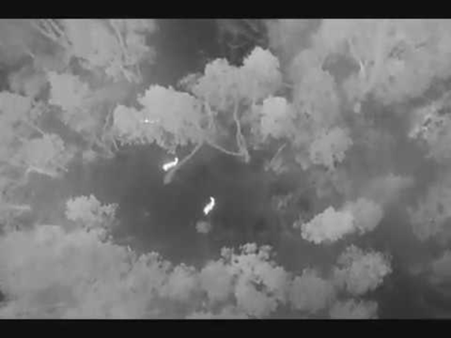
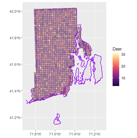
Objective: Evaluate sample size trade-offs for estimating white-tailed deer abundance throughout Rhode Island.

Methodology: Count deer in 1 sq. mile cells using FLIR technology attached to a helicopter.

Lab Setup

Steps to consider

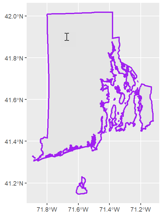
Sampling Frame
- all of RI or some subset

Lab Setup

Steps to consider

“Truth”
- how many deer per cell; how variable

Lab Setup

Steps to consider

Sampling Process
- how to pick each cell

Lab Setup

Steps to consider

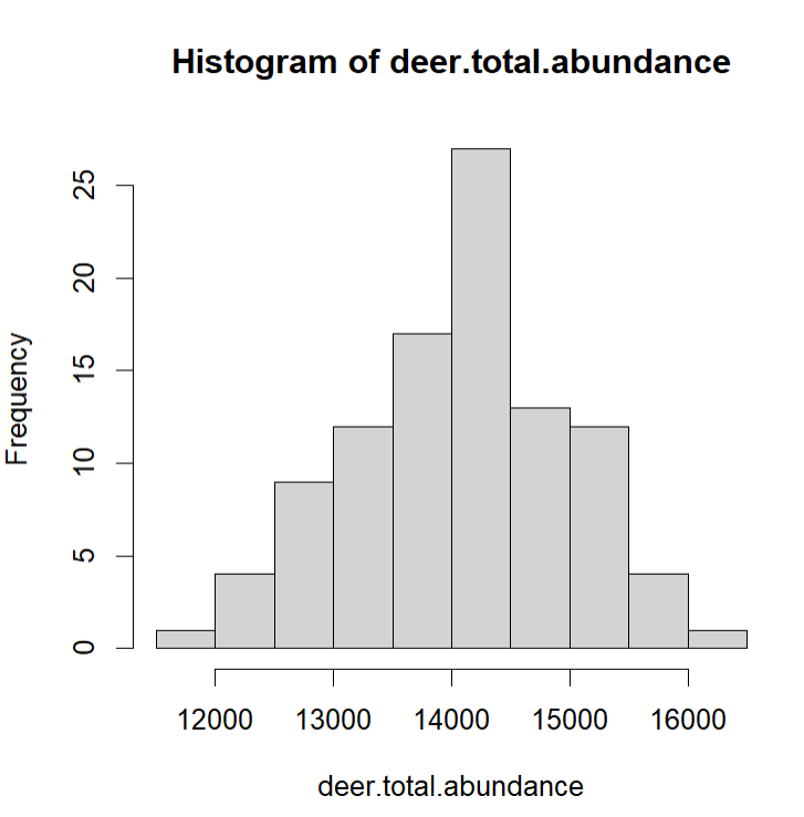
Estimation Process
- estimate total deer population from the sample
Criteria to Evaluate
- use sampling distribution of deer abundance estimate or some other statistic

Big Picture Science and Modeling

What’s the point of statistics?

Today

Study Objective

Hypothesis

Research/Scientific Hypothesis

Statistical Model/Hypothesis

Statistical Model/Hypothesis

Statistical Model/Hypothesis

Evidence of hypothesis support

Prediction

Types of Studies

Manuscript Writing

Take-Aways?

Big Data Problems

Big Data Problems

Big Data Problems

Big Data Problems

Big Data Problems

The Questioning Scientist

Data vs. Information

Information

The question and the data

The goal of the question

Take-Aways

Which is worse?

Inference and Prediction

Inference and Prediction

Inference and Prediction

Inference and Prediction

Take-Aways

Design-Based

Design-Based

Design-Based

Design-Based

Design-Based

Design-Based

Random Variable

Statistic

Design-Based Code

TRUTH

Design-Based Code

Random Sampling

Estimator for the population mean

Design-Based Code

Sampling Distribution

Design-Based Code

Design-Based Code

Design-Based Code

Model-Based

Model-Based

Model-Based

Model-Based

Model-Based Code

Model-Based Code

Model-Based Code

Sampling Distribution

Statistical Bias

Statistical Bias (Code)

Precision of the mean (Code)

Take-Aways

Lab

Lab Setup

Lab Setup

Lab Setup

Lab Setup

Lab Setup

Go to code

Big Picture
Science and Modeling