Bayes the way

All things Bayesian

  • Bayesian Inference

  • Bayes Theorem

  • Bayesian Components

    • likelihood, prior, evidence, posterior
  • Conjugacy

  • Hippo Case Study

  • Bayesian Computation


Bayesian Inference

Probability, Data, and Parameters

What do we want our model to tell us?

Do we want to make probability statements about our data?


Likelihood = P(data|parameters)


90% CI: the long-run proportion of re-sampling a population such that considering all the CI’s will contain the true value 90% of the time.

Probability, Data, and Parameters

What do we want our model to tell us?

Do we want to make probability statements about our parameters?


Posterior = P(parameters|data)


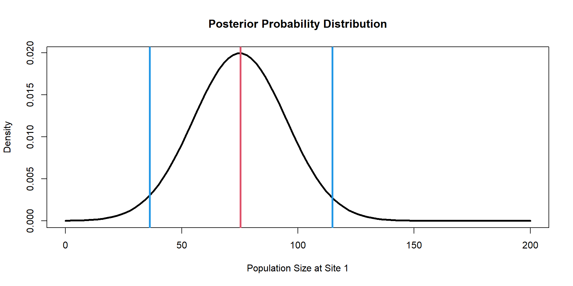
Alternative Interval: 90% probability that the true value lies within the interval, given the evidence from the observed data.

Likelihood Inference

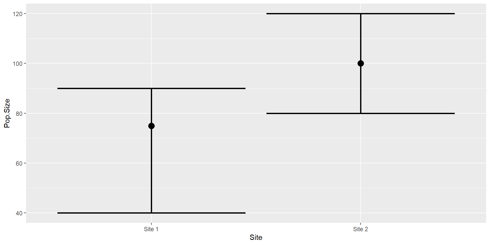
Estimate of the population size of hedgehogs at two sites.

Site Pop.Size lowerCI upperCI
Site 1 75 40 90
Site 2 100 80 120

Bayesian Inference

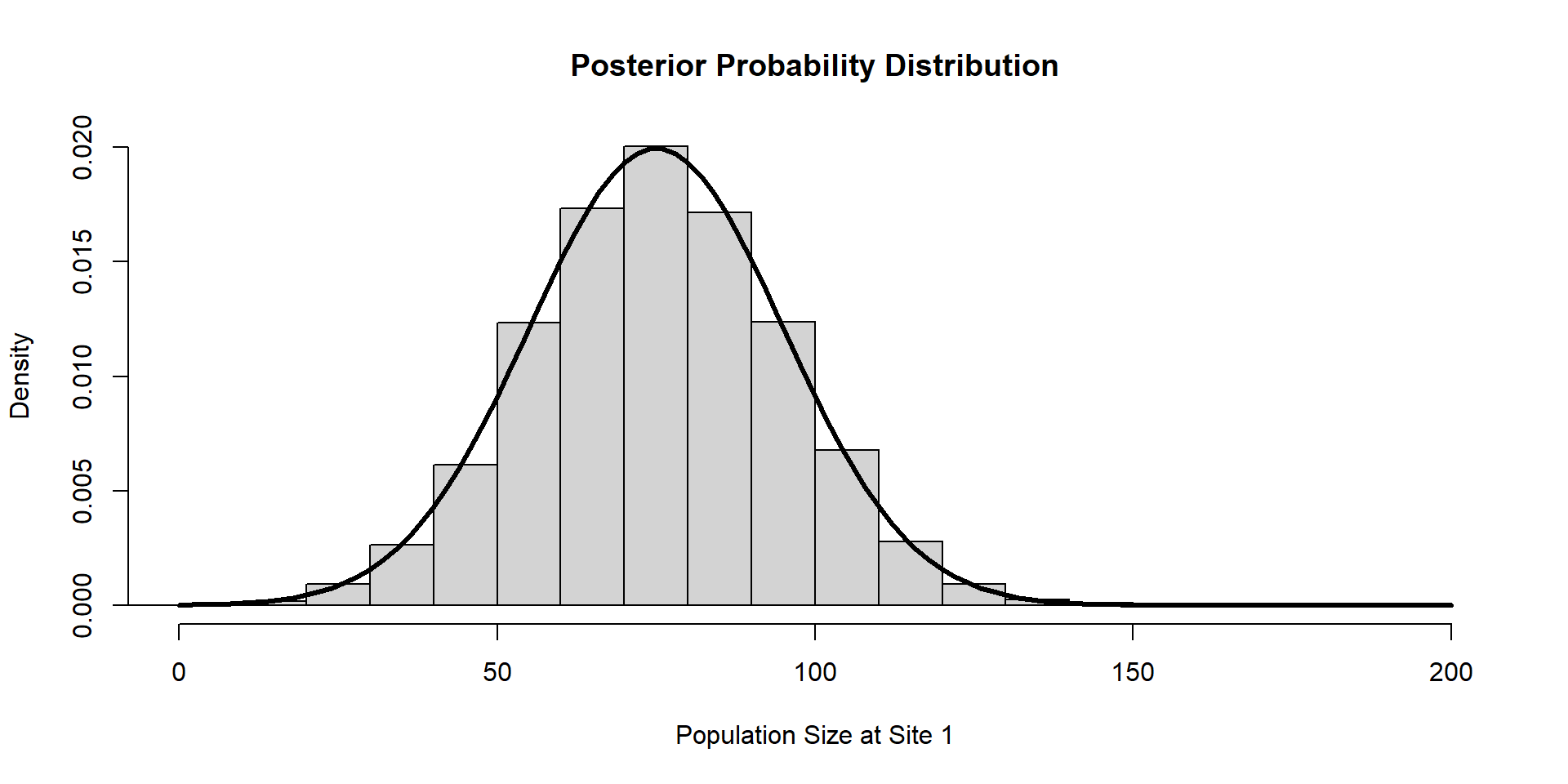
Posterior Samples

 [1] 102.67671  81.11546  81.75260  87.77246  73.99043  80.70631  76.26219
 [8]  83.99927  64.74208  26.93133

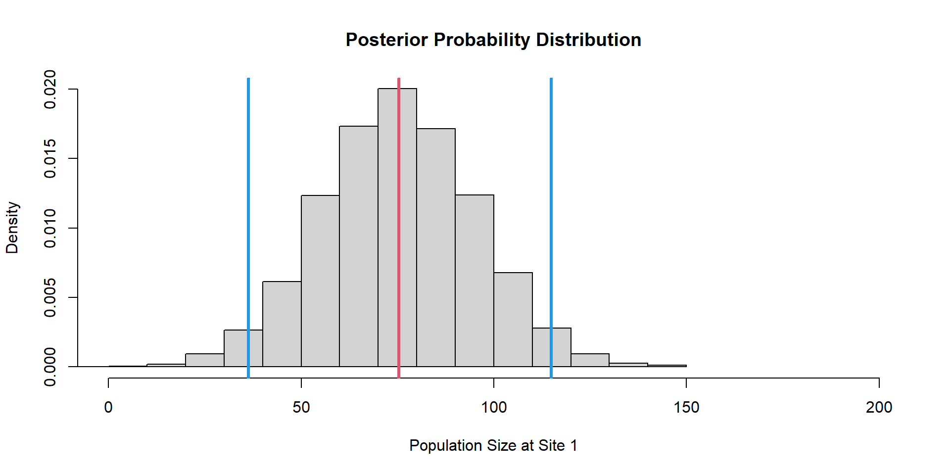
Bayesian Inference

Posterior Samples

 [1] 102.67671  81.11546  81.75260  87.77246  73.99043  80.70631  76.26219
 [8]  83.99927  64.74208  26.93133

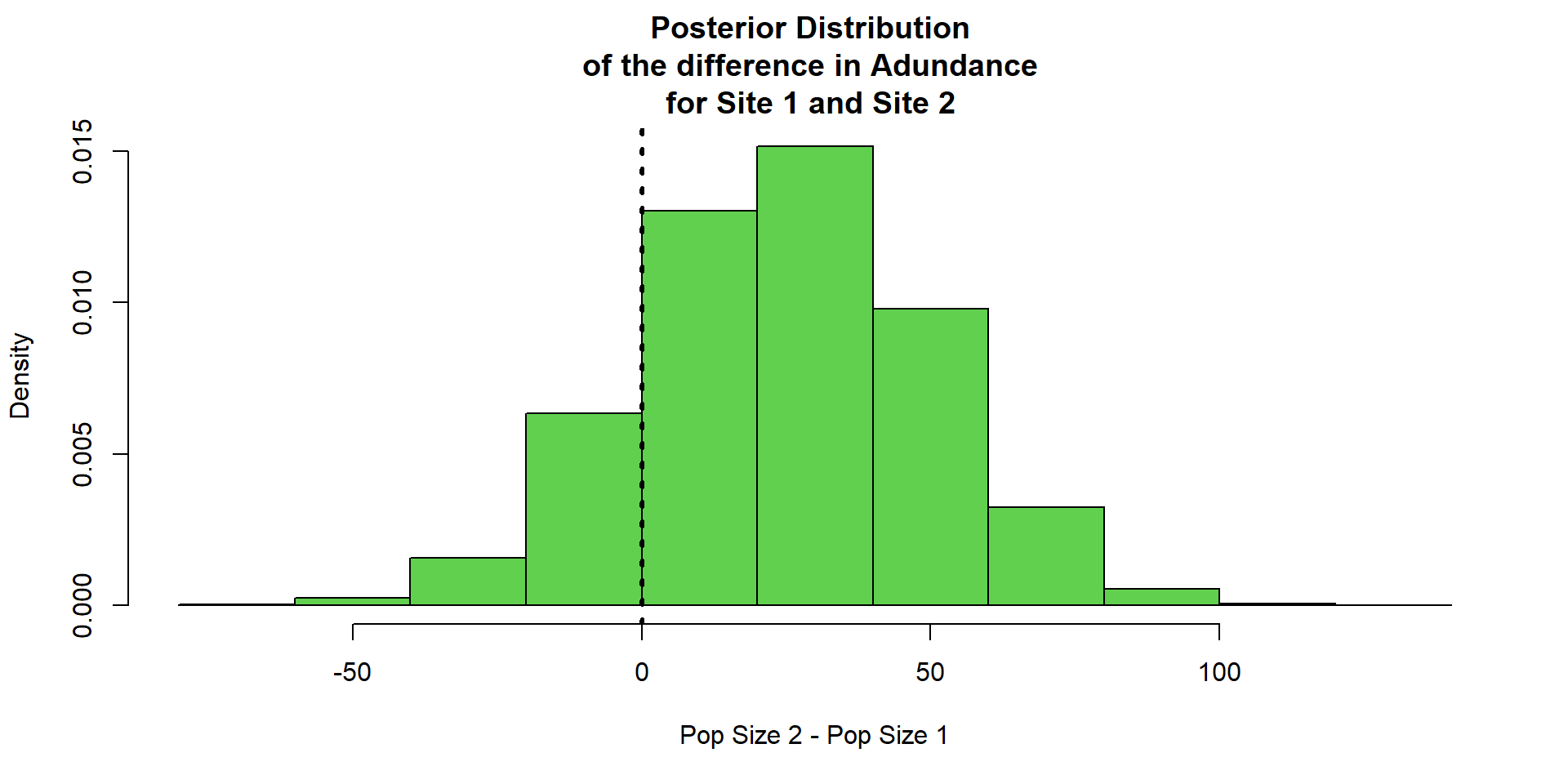
Bayesian Inference

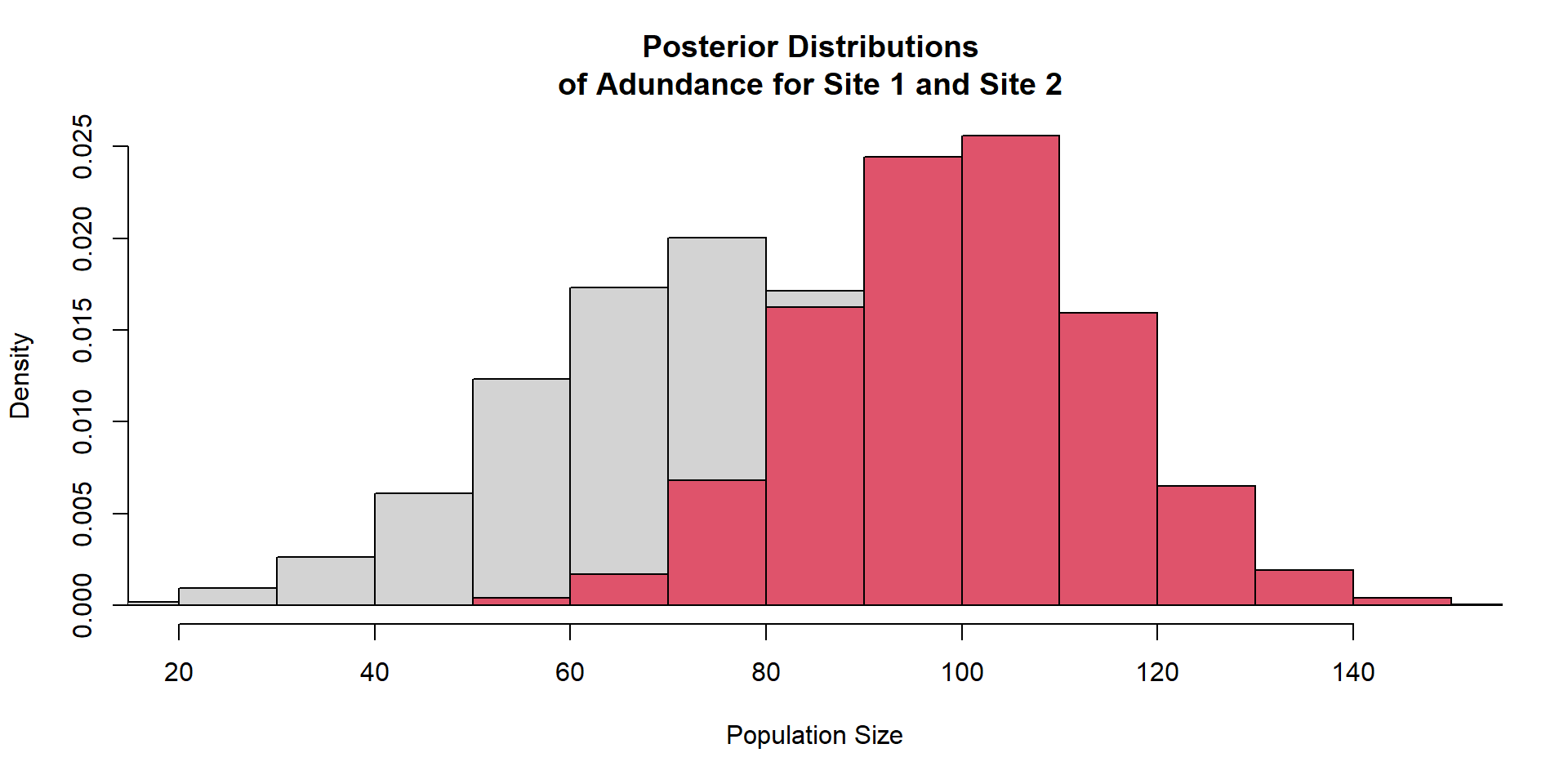
Bayesian Inference

diff = post2 - post1

P(Pop Size 2 > Pop Size 1) =

length(which(diff>0))/length(diff)
[1] 0.8362

Likelihood Inference (coefficient)

y is Body size of a beetle species

x is elevation

Interpret the p-values…

summary(glm(b.size~elev))

Call:
glm(formula = b.size ~ elev)

Coefficients:
            Estimate Std. Error t value Pr(>|t|)    
(Intercept)   0.9862     0.2435   4.049 0.000684 ***
elev          0.5089     0.4022   1.265 0.221093    
---
Signif. codes:  0 '***' 0.001 '**' 0.01 '*' 0.05 '.' 0.1 ' ' 1

(Dispersion parameter for gaussian family taken to be 1.245548)

    Null deviance: 25.659  on 20  degrees of freedom
Residual deviance: 23.665  on 19  degrees of freedom
AIC: 68.105

Number of Fisher Scoring iterations: 2

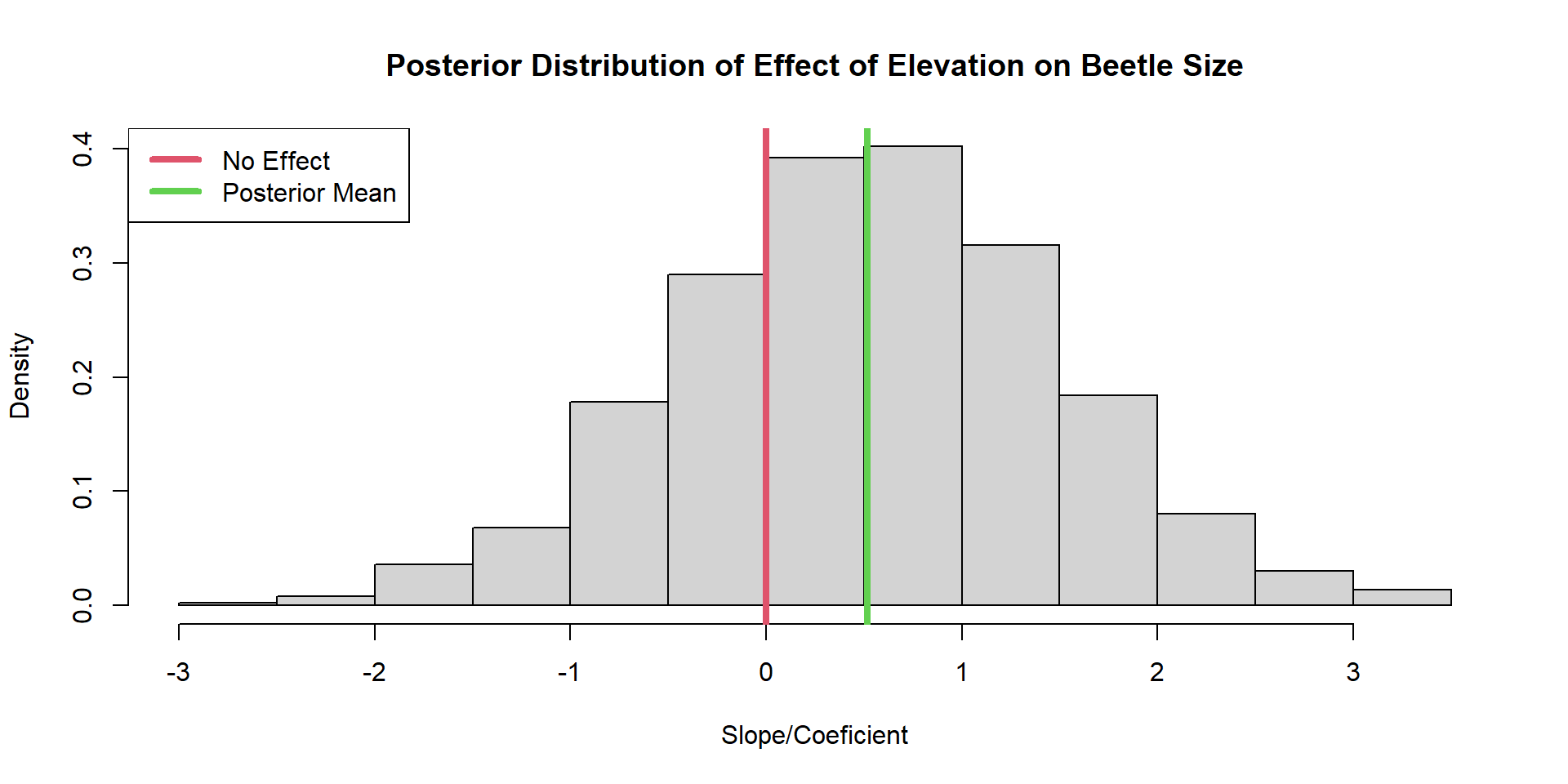
Bayesian Inference (coefficient)

Describing the posterior

Central Tendency:

  mean(post)
[1] 0.5185186
  quantile(post,prob=0.5)
      50% 
0.5319192 
  modeest::shorth(post)
[1] 0.5438012

Describing the posterior

Probability Intervals

# Quantile Credible Intervals:
  quantile(post,
           prob = c(0.025,0.975)
           )
     2.5%     97.5% 
-1.461887  2.403232 
# Highest Posterior Density Intervals (HPDI)
  coda::HPDinterval(coda::as.mcmc(post),
                    prob = 0.95
                    )
         lower    upper
var1 -1.534921 2.283981
attr(,"Probability")
[1] 0.95

Describing the posterior

Derived Probabilities

# Probability of a positive effect (exact p-value)
 length(which(post>0))/length(post)
[1] 0.709
# Probability of a negative effect (exact p-value)
 length(which(post<0))/length(post)
[1] 0.291


Bayesian Theorem

Bayes Theorem

Link

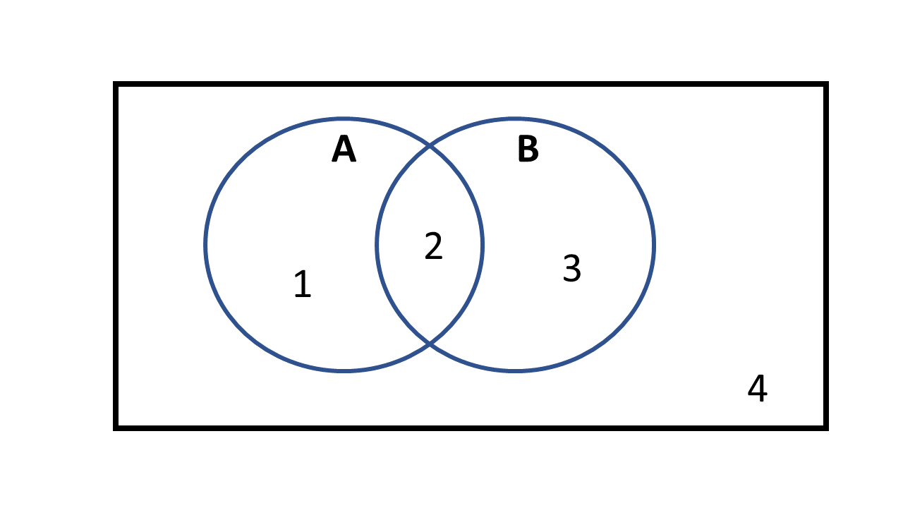
  • Marginal Probability

    • \(P(A)\)
    • \(P(B)\)
Click for Answer
# P(A)
3/10 = 0.3

# P(B)
5/10 = 0.5
Sampled N = 10 locations

Bayes Theorem

  • Joint Probability

    • \(P(A \cap B)\)
Click for Answer
# P(A and B)
2/10 = 0.2
Sampled N = 10 locations

Bayes Theorem

  • Conditional Probability

    • \(P(A|B)\)
    • \(P(B|A)\)
Click for Answer
# P(A|B)
2/5 = 0.4

# P(B|A)
2/3 = 0.6666
Sampled N = 10 locations

Bayes Theorem

  • OR Probability

    • \(P(A\cup B)\)
Click for Answer
# P(A or B)
# P(A) + P(B) - P(A and B)

0.3 + 0.5 - 0.2 = 0.6
Sampled N = 10 locations

Notice that…

\[ \begin{equation} P(A \cap B) = 0.2 \\ P(A|B)P(B) = 0.4 \times 0.5 = 0.2 \\ P(B|A)P(A) = 0.6666 \times 0.3 = 0.2 \\ \end{equation} \]

\[ \begin{equation} P(A|B)P(B) = P(A \cap B) \\ P(B|A)P(A) = P(A \cap B) \\ \end{equation} \]

\[ \begin{equation} P(B|A)P(A) = P(A|B)P(B) \end{equation} \]

Bayes Theoreom

\[ \begin{equation} P(B|A) = \frac{P(A|B)P(B)}{P(A)} \\ \end{equation} \]

\[ \begin{equation} P(B|A) = \frac{P(A \cap B)}{P(A)} \\ \end{equation} \]


Bayesian Components

Bayes Components

param = parameters \[ \begin{equation} P(\text{param}|\text{data}) = \frac{P(\text{data}|\text{param})P(\text{param})}{P(\text{data})} \\ \end{equation} \]

Posterior Probability/Belief

Likelihood

Prior Probability

Evidence or Marginal Likelihood

Bayes Components

param = parameters

\[ \begin{equation} P(\text{param}|\text{data}) = \frac{P(\text{data}|\text{param})P(\text{param})}{\int_{\forall \text{ Param}} P(\text{data}|\text{param})P(\text{param})} \end{equation} \]

Posterior Probability/Belief

Likelihood

Prior Probability

Evidence or Marginal Likelihood

Bayes Components

\[ \begin{equation} \text{Posterior} = \frac{\text{Likelihood} \times \text{Prior}}{\text{Evidence}} \\ \end{equation} \]

\[ \begin{equation} \text{Posterior} \propto \text{Likelihood} \times \text{Prior} \end{equation} \]

\[ \begin{equation} \text{Posterior} \propto \text{Likelihood} \end{equation} \]

The Prior

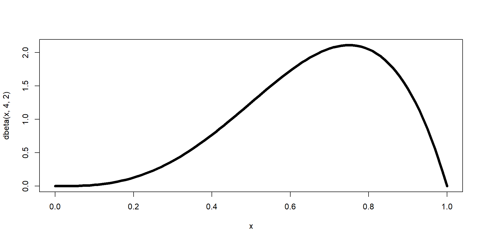
All parameters in a Bayesian model require a prior specified; parameters are random variables.

\(y_{i} \sim \text{Binom}(N, p)\)

\(p \sim \text{Beta}(\alpha = 4, \beta=2)\)

curve(dbeta(x, 4,2),xlim=c(0,1),lwd=5)

The Prior

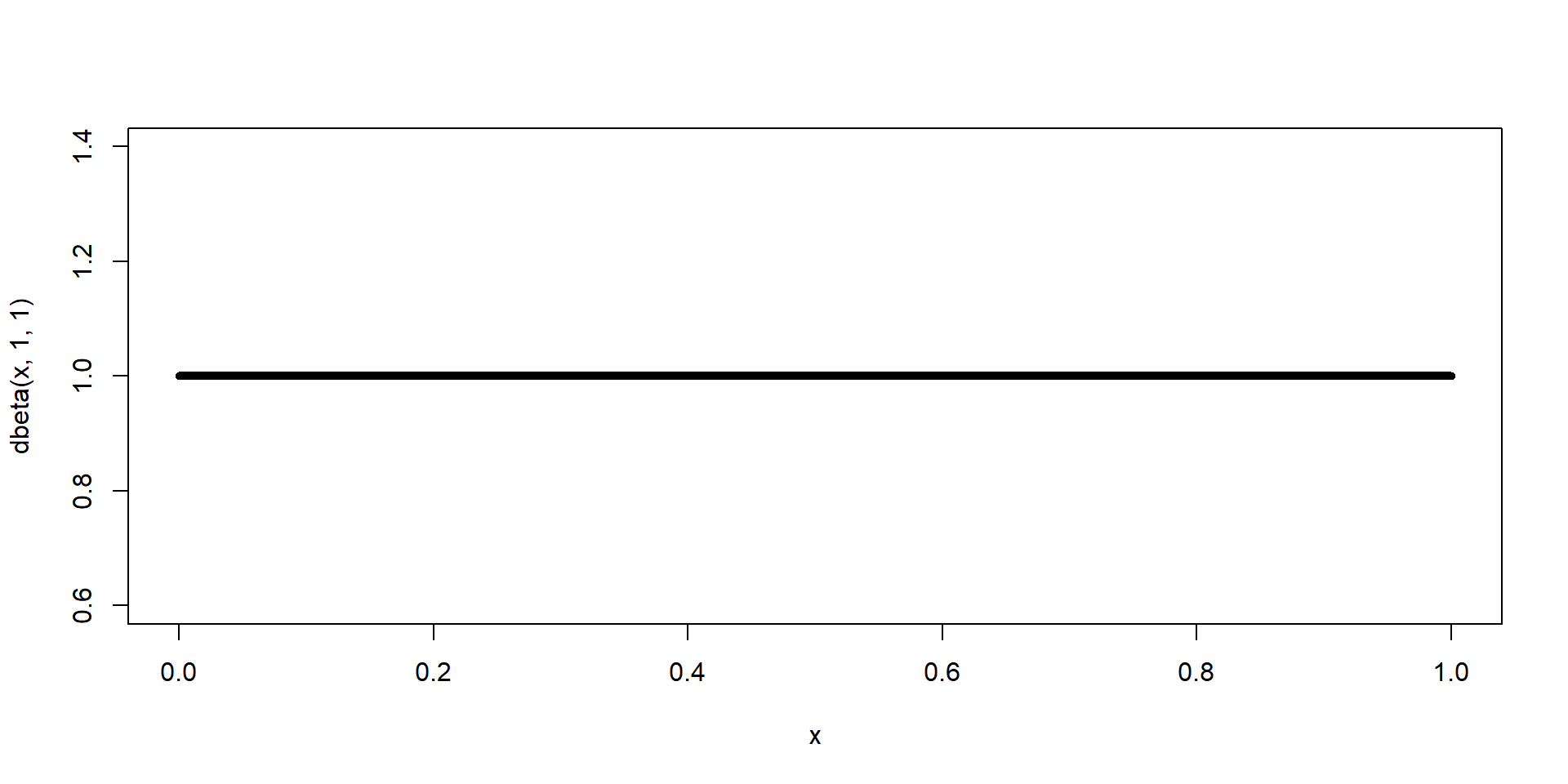
\(p \sim \text{Beta}(\alpha = 1, \beta=1)\)

curve(dbeta(x, 1,1),xlim=c(0,1),lwd=5)

The Prior

  • The prior describes what we know about the parameter before we collect any data

  • Priors can contain a lot of information (informative priors ) or very little (diffuse priors )

  • Well-constructed priors can also improve the behavior of our models (computational advantage)

  • No such thing as a ‘non-informative’ prior

  • Diffuse priors on one scale can be very informative on another

The Prior

Use diffuse priors as a starting point

It’s fine to use diffuse priors as you develop your model but you should always prefer to use “appropriate, well-contructed informative priors” (Hobbs & Hooten, 2015)

The Prior

Use your “domain knowledge”

We can often come up with weakly informative priors just by knowing something about the range of plausible values of our parameters.

The Prior

Dive into the literature

Find published estimates and use moment matching and other methods to convert published estimates into prior distributions

The Prior

Visualize your prior distribution

Be sure to look at the prior in terms of the parameters you want to make inferences about (use simulation!)

The Prior

Do a sensitivity analysis

Does changing the prior change your posterior inference? If not, don’t sweat it. If it does, you’ll need to return to point 2 and justify your prior choice

The Prior

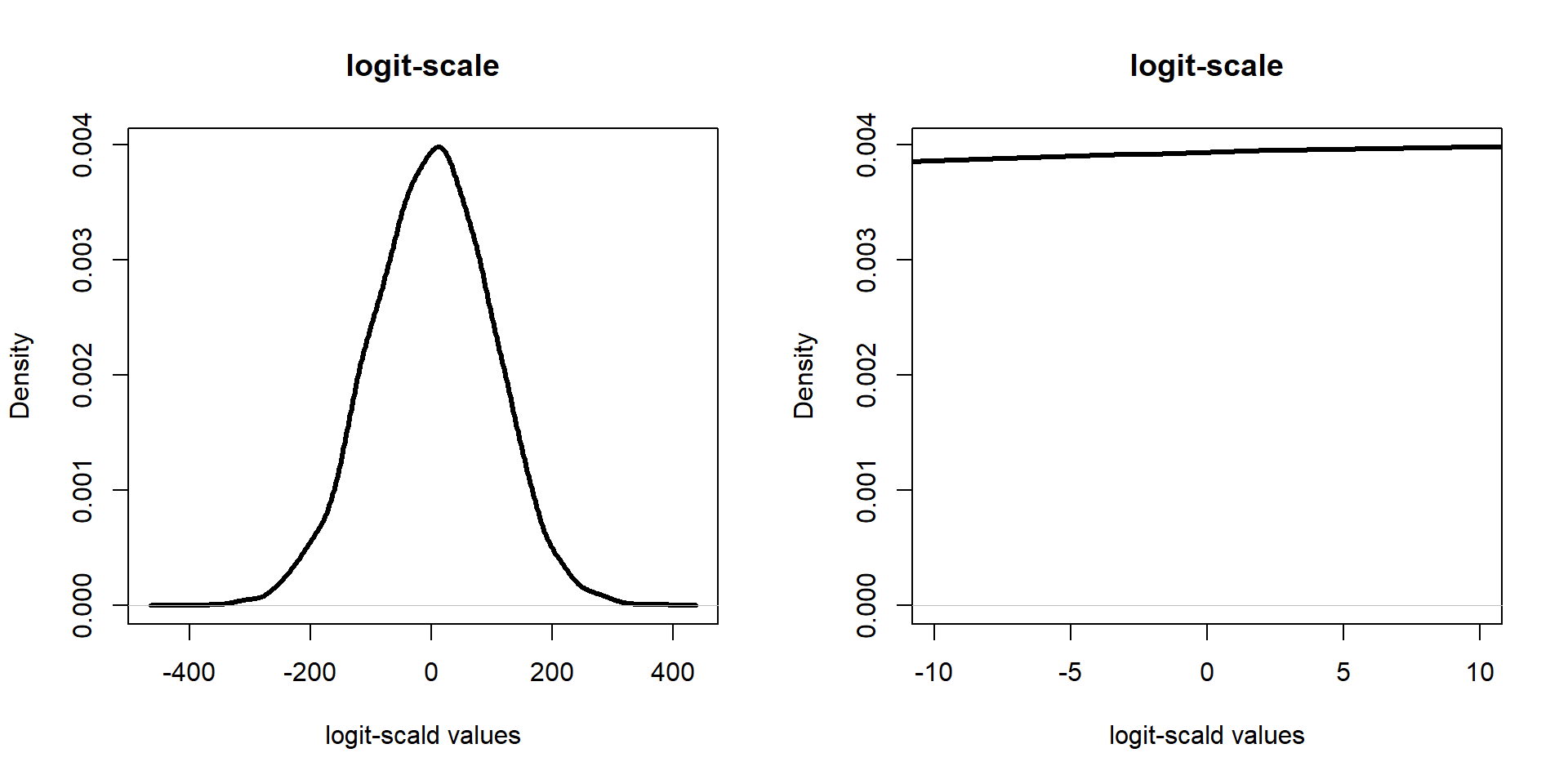
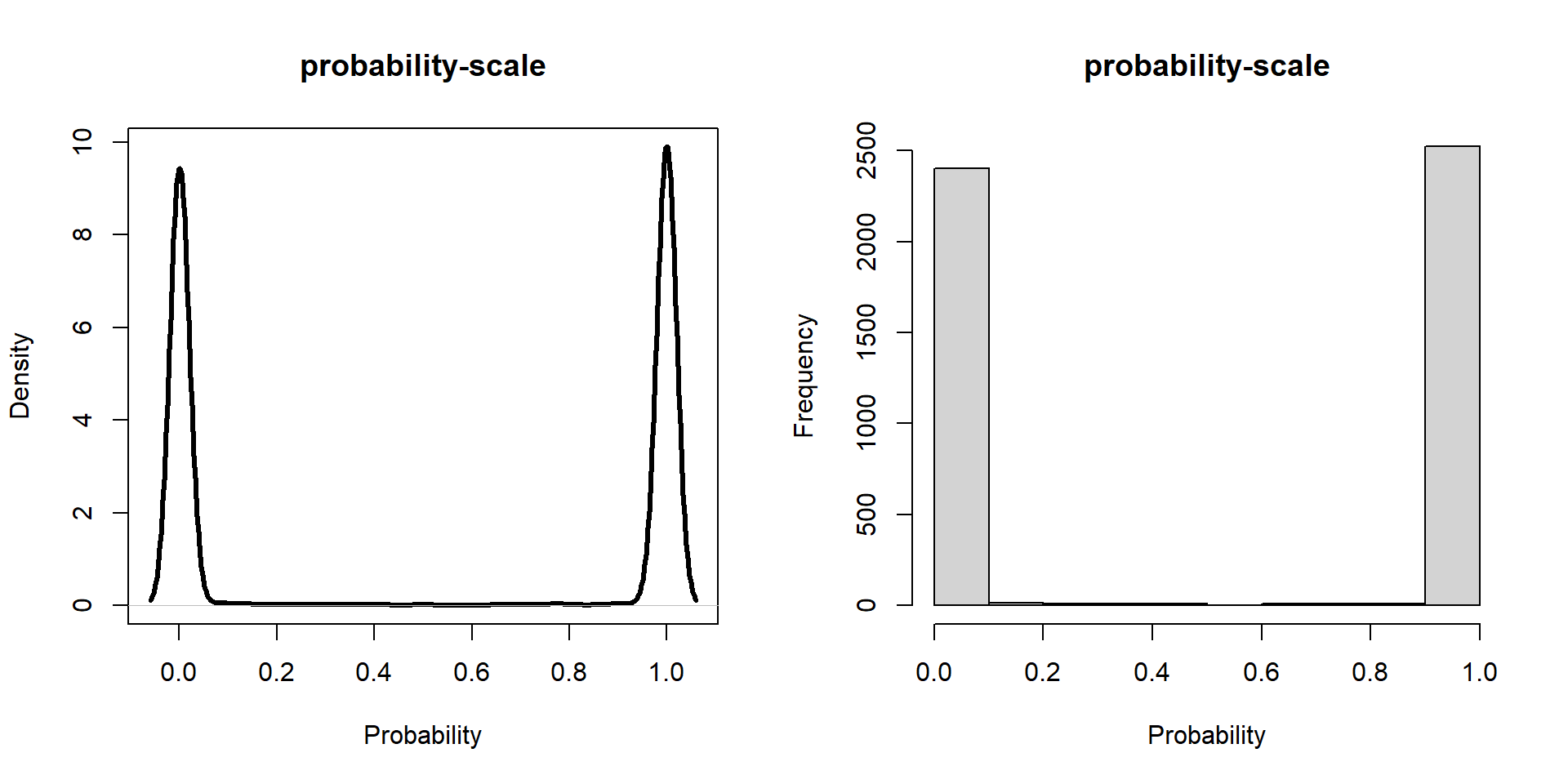
Priors are mostly not invariant to transformation of scale

\[ \begin{align*} \textbf{y}_{i} \sim& \text{Bernoulli}(p_{i})\\ \text{logit}(p_{i}) =& \beta_0\\ \beta_0 \sim& \text{Normal(0,100)} \end{align*} \]

The Prior

Priors are mostly not invariant to transformation of scale

The Prior

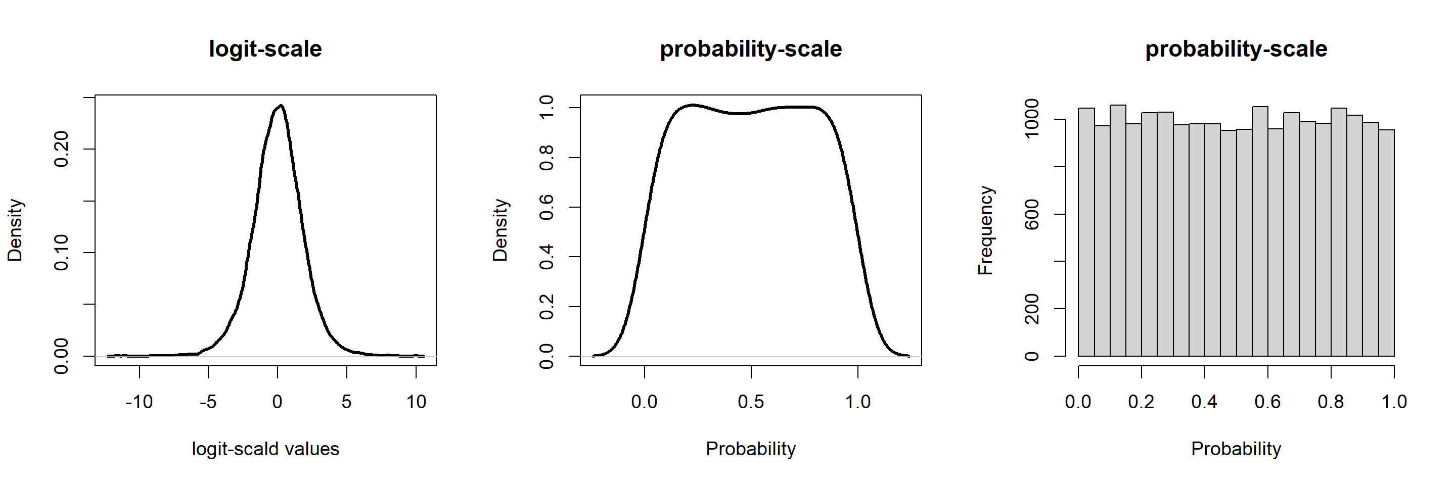
There are intermediate solutions

\[ \begin{align*} \beta_0 \sim& \text{Logistic(0,1)} \end{align*} \]

Link


Conjugacy

Bayesian Model

Model

\[ \textbf{y} \sim \text{Bernoulli}(p) \]

Prior

\[ p \sim \text{Beta}( \alpha, \beta) \\ \]

These are called Prior hyperparameters

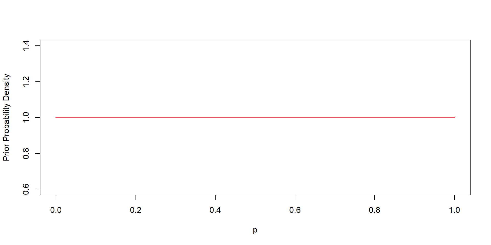
\[ \alpha = 1 \\ \beta = 1 \]

curve(dbeta(x,1,1),xlim=c(0,1),lwd=3,col=2,xlab="p",
      ylab = "Prior Probability Density")

Conjugate Distribution

Likelihood (Joint Probability of y)

\[ \mathscr{L}(p|y) = \prod_{i=1}^{n} P(y_{i}|p) = \prod_{i=1}^{N}(p^{y}(1-p)^{1-y_{i}}) \]

Prior Distribution

\[ P(p) = \frac{p^{\alpha-1}(1-p)^{\beta-1}}{B(\alpha,\beta)} \]

Posterior Distribution of p

\[ P(p|y) = \frac{\prod_{i=1}^{N}(p^{y}(1-p)^{1-y_{i}}) \times \frac{p^{\alpha-1}(1-p)^{\beta-1}}{B(\alpha,\beta)} }{\int_{p}(\text{numerator})} \]

CONJUGACY!

\[ P(p|y) \sim \text{Beta}(\alpha^*,\beta^*) \]

\(\alpha^*\) and \(\beta^*\) are called Posterior hyperparameters

\[ \alpha^* = \alpha + \sum_{i=1}^{N}y_i \\ \beta^* = \beta + N - \sum_{i=1}^{N}y_i \\ \]

Wikipedia Conjugate Page

Conjugate Derivation


Case Study

Hippos

We do a small study on hippo survival and get these data…

7 Hippos Died
2 Hippos Lived

Hippos: Likelihood Model

\[ \begin{align*} \textbf{y} \sim& \text{Binomial}(N,p)\\ \end{align*} \]

# Survival outcomes of three adult hippos
  y1 = c(0,0,0,0,0,0,0,1,1)
  N1 = length(y1)
  mle.p = mean(y1)
  mle.p
[1] 0.2222222

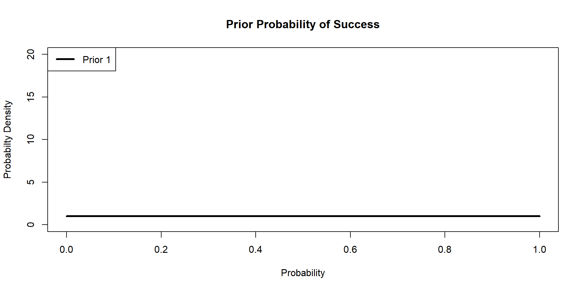
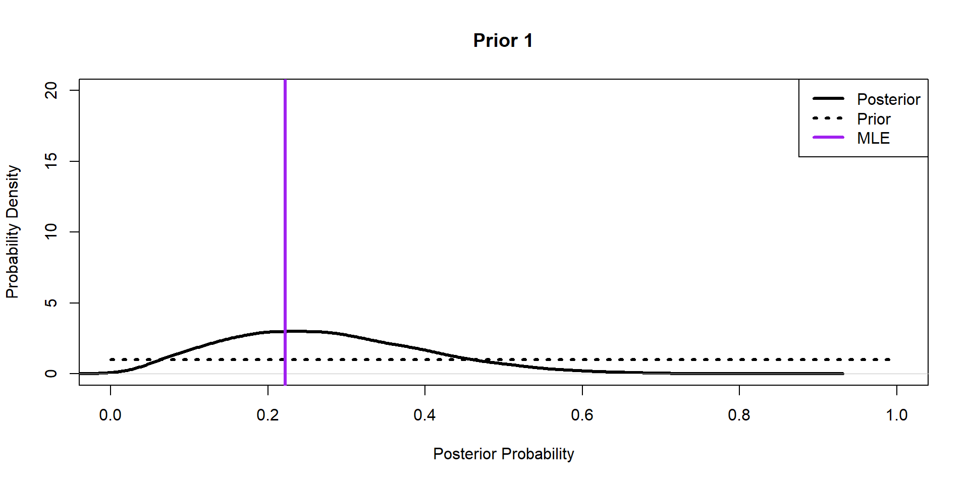
Hippos: Bayesian Model (Prior 1)

\[ \begin{align*} \textbf{y} \sim& \text{Binomial}(N,p)\\ p \sim& \text{Beta}(\alpha,\beta) \end{align*} \]

  alpha.prior1 = 1
  beta.prior1 = 1

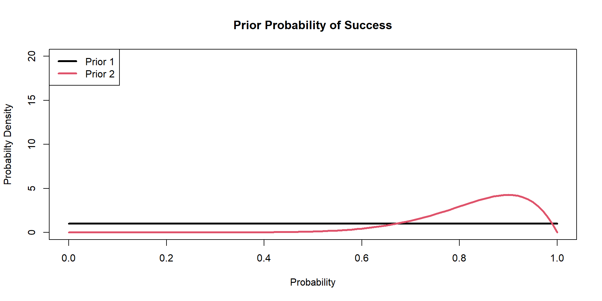
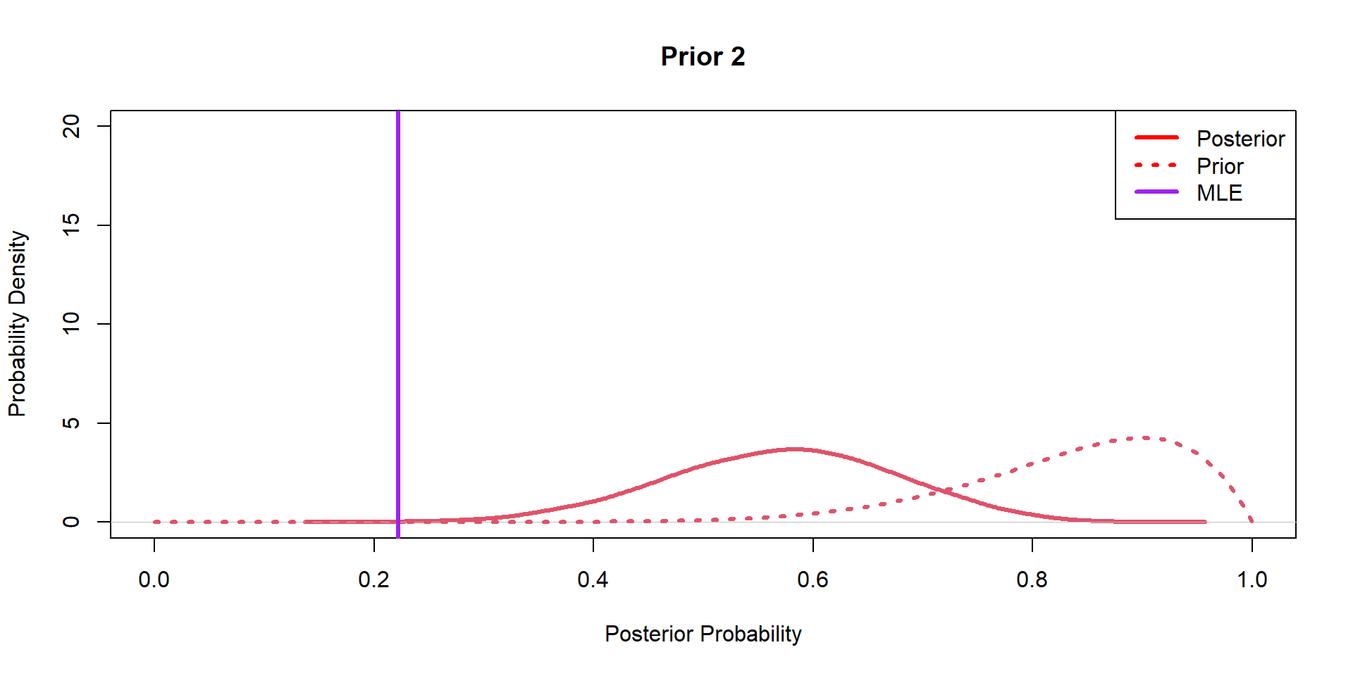
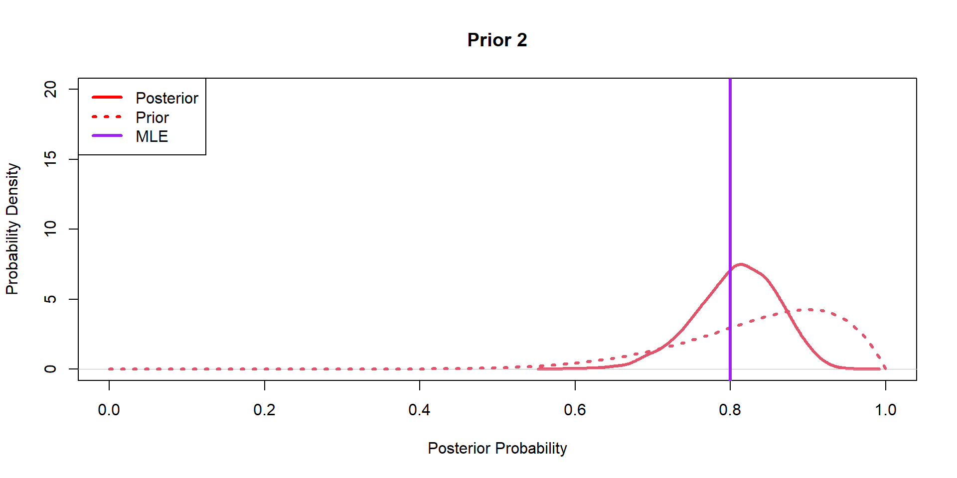
Hippos: Bayesian Model (Prior 2)

  alpha.prior2 = 10
  beta.prior2 = 2

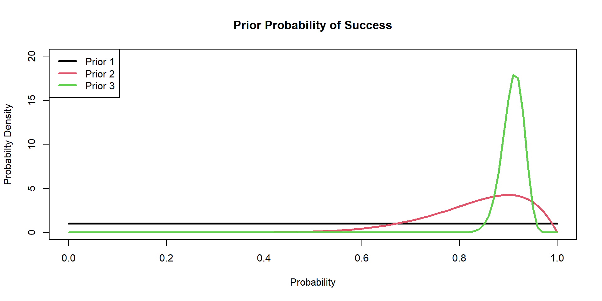
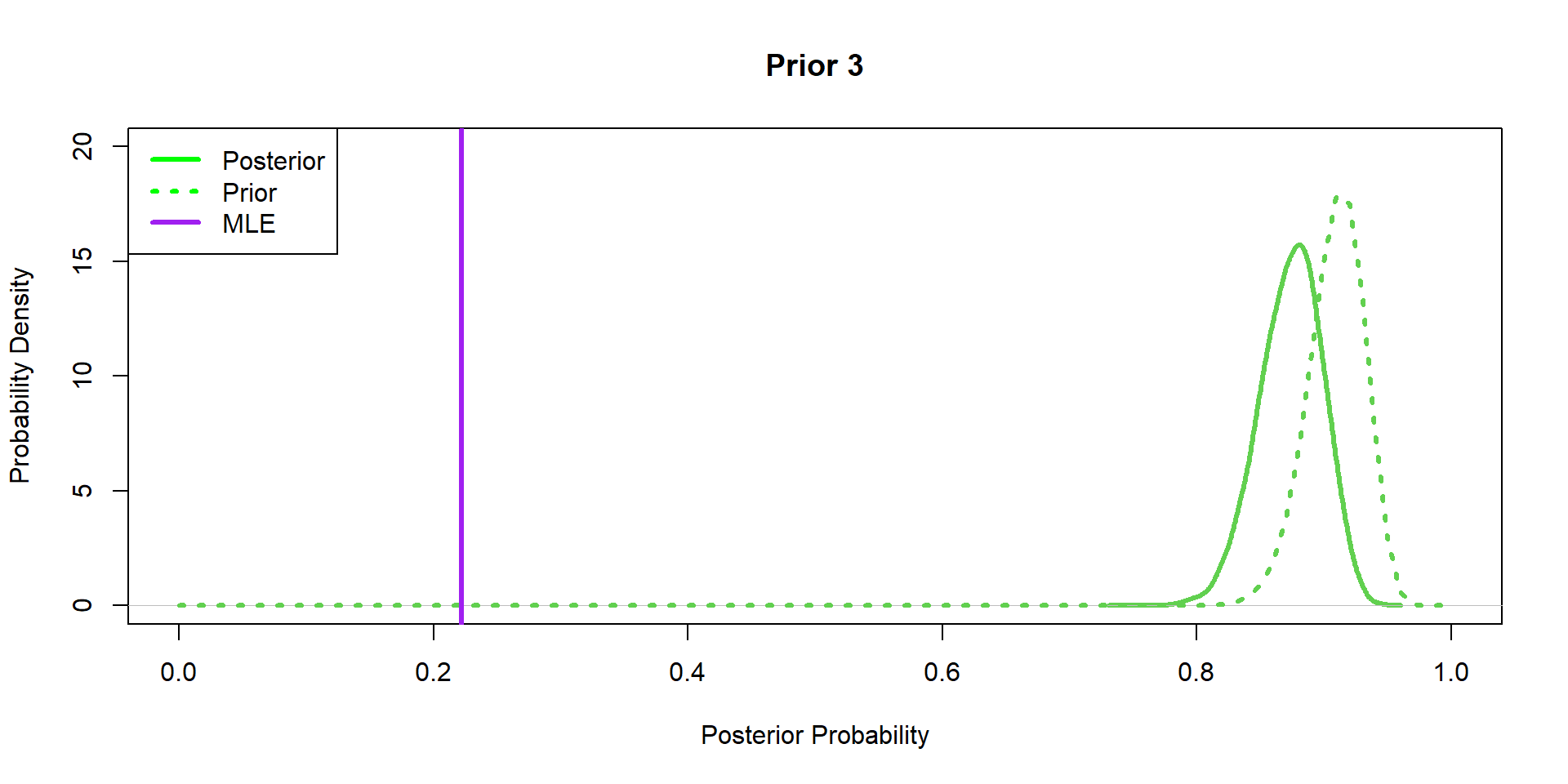
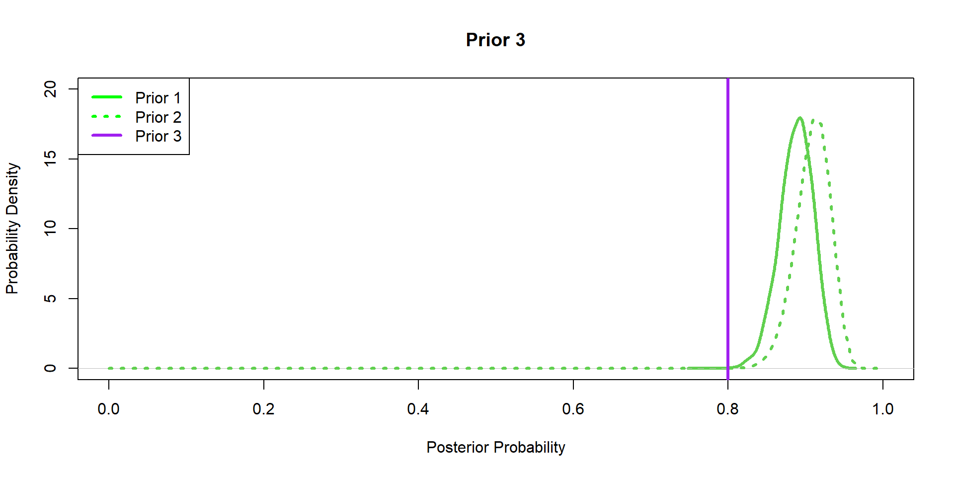
Hippos: Bayesian Model (Prior 3)

  alpha.prior3 = 150
  beta.prior3 = 15

Hippos: Bayesian Model (Posteriors)

\[ P(p|y) \sim \text{Beta}(\alpha^*,\beta^*)\\ \alpha^* = \alpha + \sum_{i=1}^{N}y_i \\ \beta^* = \beta + N - \sum_{i=1}^{N}y_i \\ \]

# Note how the data are the same, but the prior is changing.
# Gibbs sampler
  post.1 = rbeta(10000,alpha.prior1+sum(y1),beta.prior1+N1-sum(y1))
  post.2 = rbeta(10000,alpha.prior2+sum(y1),beta.prior2+N1-sum(y1))
  post.3 = rbeta(10000,alpha.prior3+sum(y1),beta.prior3+N1-sum(y1))
Hippos: Bayesian Model (Posteriors)

Hippos: Bayesian Model (Posteriors)

Hippos: Bayesian Model (Posteriors)

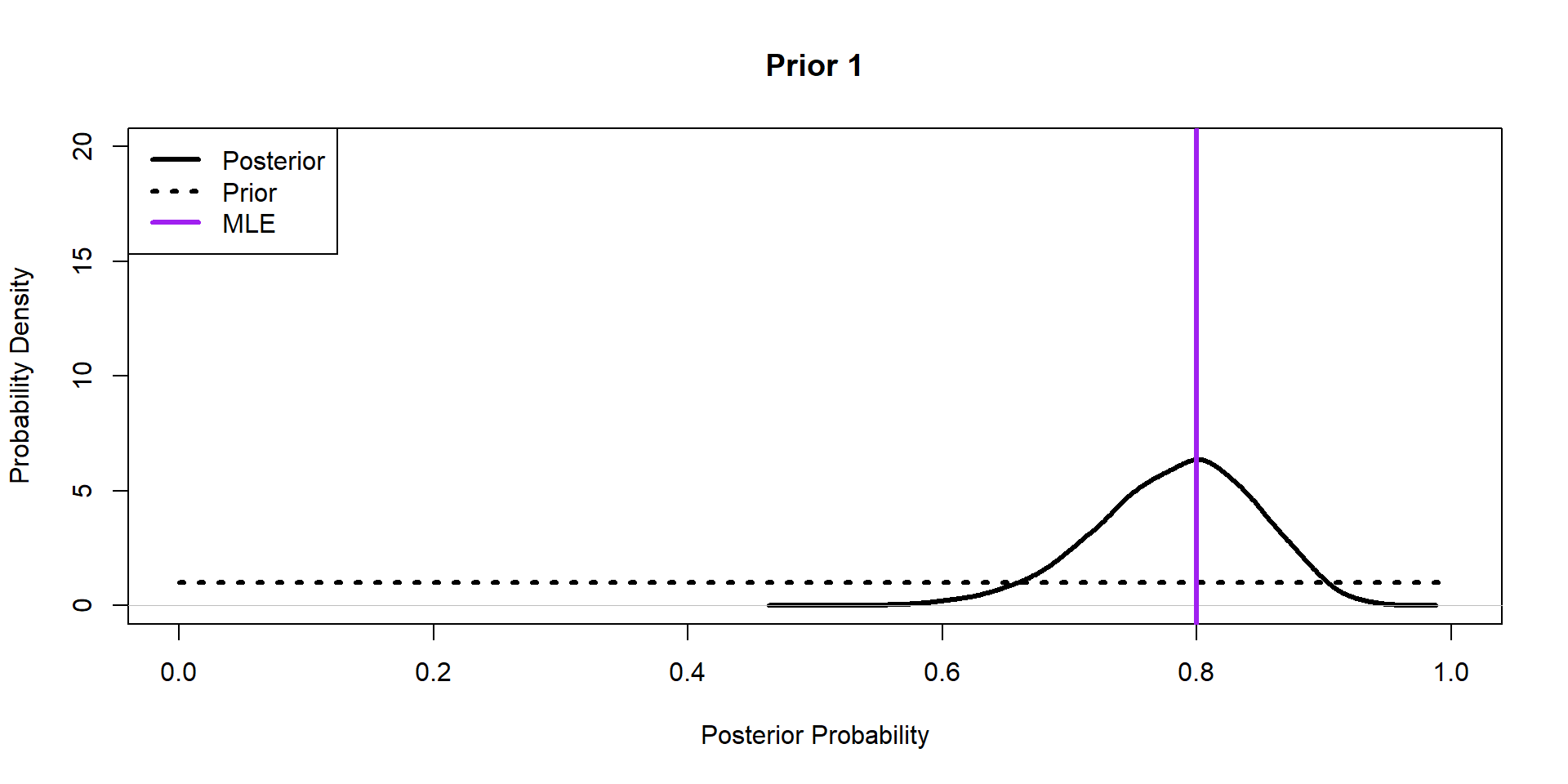
Hippos: More data! (Prior 1)

y2 = c(0,0,0,0,0,0,0,1,1,1,1,1,1,1,1,1,1,1,1,1,0,
       1,1,1,1,1,1,1,1,1,1,1,1,1,1,1,1,1,1,1)
length(y2)
[1] 40

Hippos: More data! (Prior 2)

Hippos: More data! (Prior 3)

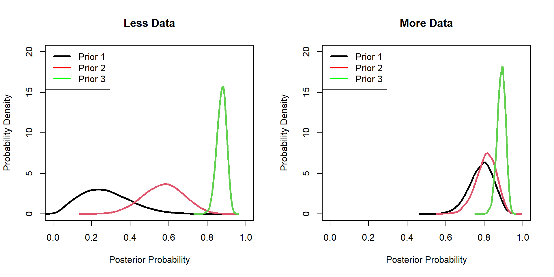
Hippos: Data/prior Comparison


Bayesian Computation

Markov Chain Monte Carlo

Often don’t have conjugate likelihood and priors, so we use MCMC algorithims to sample posteriors.

Class of algorithm

  • Metropolis-Hastings
  • Gibbs
  • Reversible-Jump
  • No U-turn Sampling

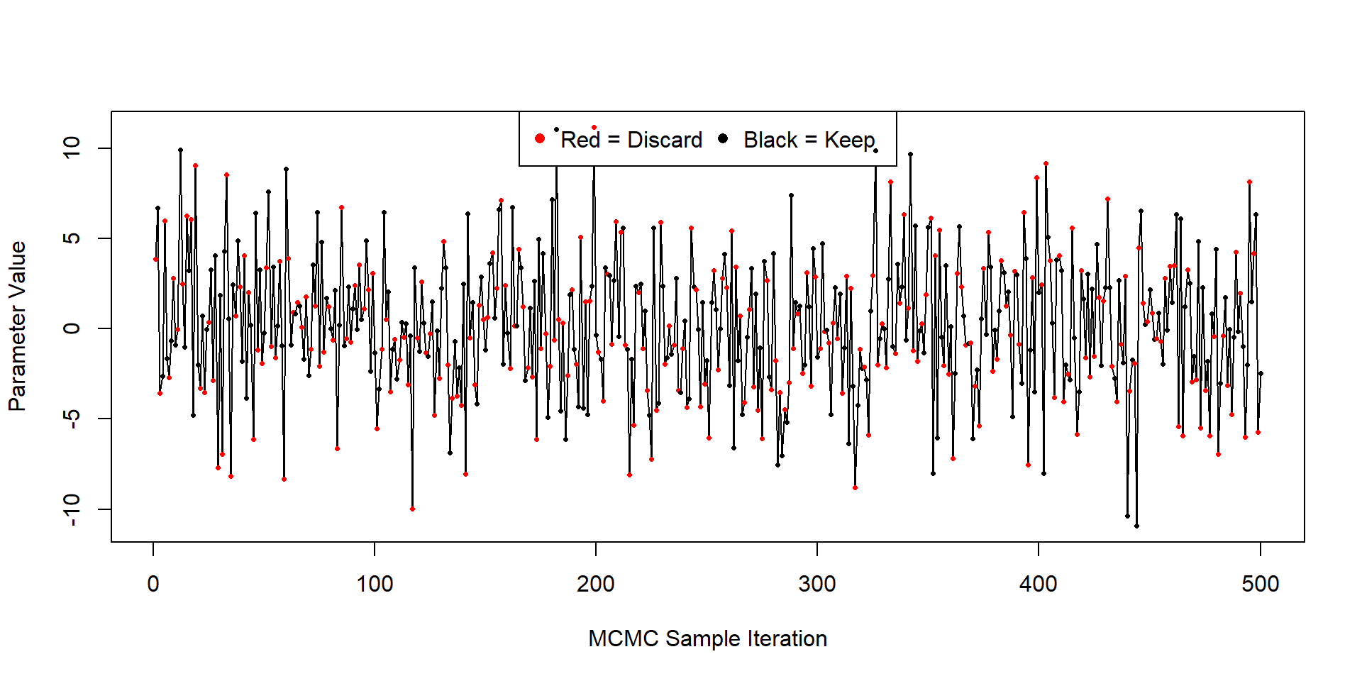
Markov Chain Monte Carlo

\[ P(p|y) = \frac{\prod_{i=1}^{N}(p^{y}(1-p)^{1-y_{i}}) \times \frac{p^{\alpha-1}(1-p)^{\beta-1}}{B(\alpha,\beta)} }{\int_{p}(\text{numerator})} \]

\[ P(p|y) \propto\prod_{i=1}^{N}(p^{y}(1-p)^{1-y_{i}}) \times \frac{p^{\alpha-1}(1-p)^{\beta-1}}{B(\alpha,\beta)} \]

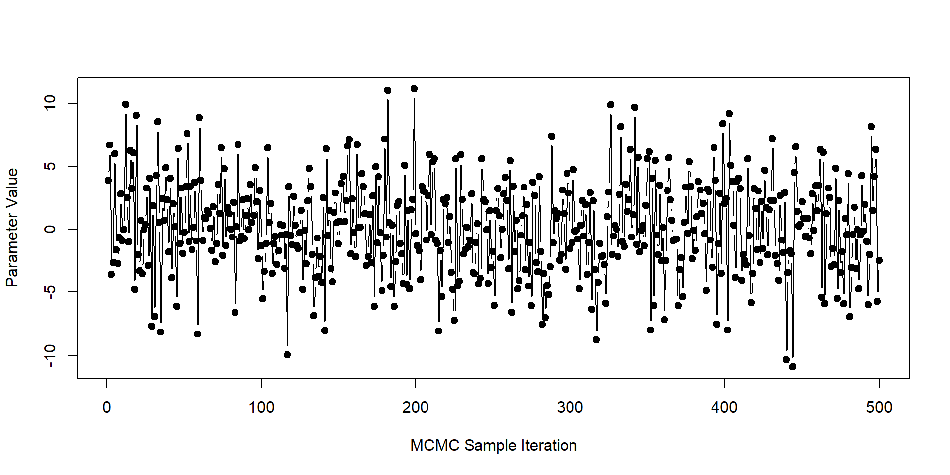
MCMC Sampling language

  • iterations: number of samples to draw/generate from a posterior distribution

MCMC Sampling language

  • thinning: which iterations to keep, every one (1), ever other one (2), every third one (3)

MCMC Sampling language

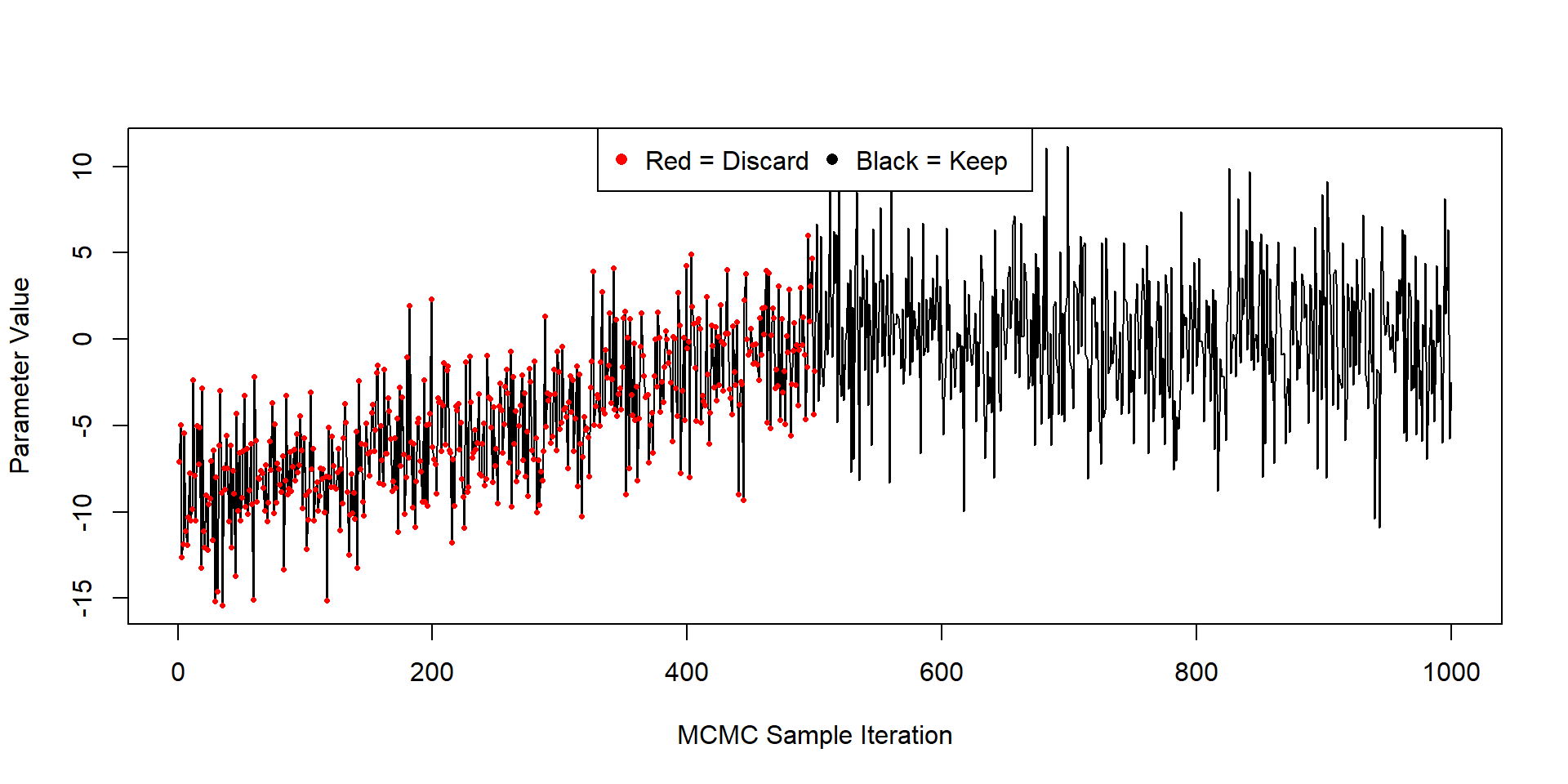
  • burn-in: how many of the initial samples to remove; depends on distance from initial value and the posterior distribution

MCMC Sampling language

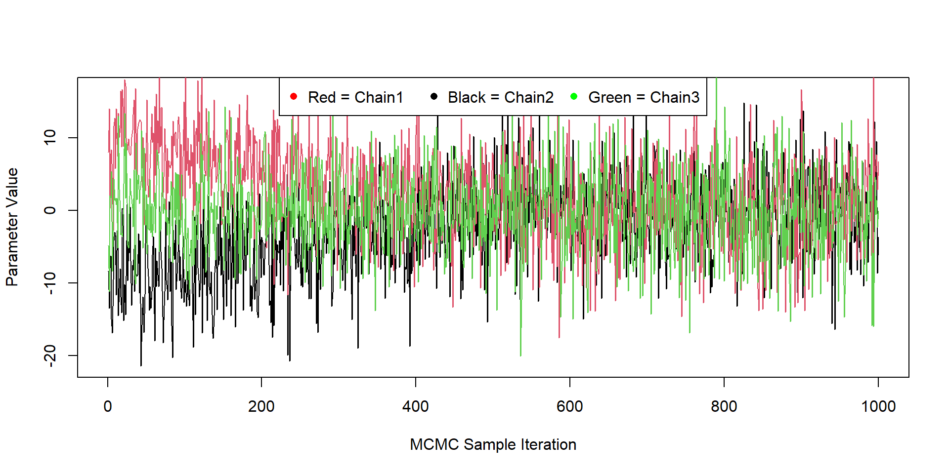
  • chains: (unique sets of samples; needed for convergence tests)

Software Options

  • Write your own algorithm
  • WinBUGS/OpenBUGS, JAGS, Stan, Nimble

Follow up

  • Bayesian Inference

  • Bayes Thereom

  • Bayesian Components

    • likelihood, prior, evidence, posterior
  • Conjugacy

  • Hippo Case Study

  • Bayesian Computation