Big Picture
Science and Modeling

What’s the point of statistics?

• a process of learning through empirical observations

• together, science philosophy and statistical modeling is the backbone to empirical learning

Today

1. Study Objectives, Hypotheses, and Predictions

2. Big Data and Sampling

3. Inference and Prediction

4. Model-Based vs Design-Based Sampling/Inference

Lab: Simulation and Markdown

Study Objective

Definition

What you want to accomplish; can have multiple related objectives in a single manuscript.

Example

To understand the space-use of coyotes.

Framing the importance of the objective(s) provides the justification and depends on the audience.

Hypothesis

Definition

1. A story that explains how the world works

2. An explanation for an observed phenomenon

Example (weak)

Coyotes have small home ranges in urban areas

Research/Scientific Hypothesis

Definition

“A statement about a phenomenon that also includes the potential mechanism or cause of that phenomenon”. (Betts et al. 2021)

Example

Coyotes have small home ranges in urban areas because food resource density is high

Non-hypothesis hypothesis: We hypothesize variation in coyote home range size.

Statistical Model/Hypothesis

Definition

• An explicit mathematical and stochastic representation of the observational & mechanistic process of the empirical observations.

Statistical Model/Hypothesis

Example:

\[\textbf{y} = \beta_0 + \beta_1 \times \textbf{x} + \mathbf{\epsilon}\] \[\mathbf{\epsilon} \sim \text{Normal}(0, \sigma^2)\]

where…

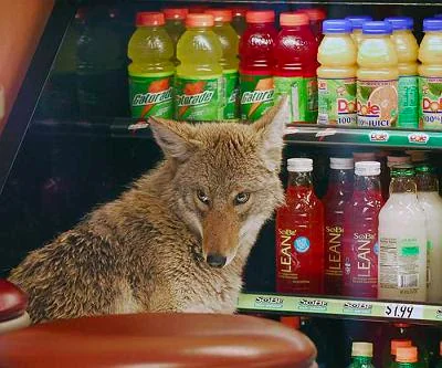
\(\textbf{y}\) = vector of home range sizes of coyotes
\(\beta_0\) = intercept
\(\beta_1\) = effect diff. of HR size for urban coyotes
\(\textbf{x}\) = indicator of HR in urban (1) or not in urban (0)
\(\sigma^2\) = uncertainty / unknown variability

Statistical Model/Hypothesis

Example:

\[\textbf{y} = \beta_0 + \beta_1 \times \textbf{x} + \mathbf{\epsilon}\] \[\mathbf{\epsilon} \sim \text{Normal}(0, \sigma^2)\]

Evidence of hypothesis support

\(\beta_1\) is negative and statistically clearly different¹ than zero

Prediction

Definition

The expected outcome from a hypothesis. If agrees with data, it would support the hypothesis or at least not reject it.

Example 1

1. Okay: Coyote home ranges are smaller in urban areas compared to non-urban areas

Example 2

2. Better: Coyote home ranges in urban areas with high available food resources is smaller than coyote home ranges in urban areas with less available food resources and smaller than coyotes living in non-urban areas

Types of Studies

• Descriptive/Naturalist (not hypothetico-deductive)

• Hypothetico-Deductive Observational

• Hypothetico-Deductive Experimental

Manuscript Writing

Where do you put these?

• objectives
• justification of objectives
• hypotheses
• predictions

Take-Aways?

1. Study Objectives, Hypotheses, and Predictions

Data is everywhere
It is the era of BIG DATA!

Big Data Problems

“The hidden Biases of Big Data” by Kate Crawford (2013)

“with enough data, the numbers speak for themselves”- Wired Magazine Editor

Big Data Problems

“The hidden Biases of Big Data” by Kate Crawford (2013)

"Data and data sets are not objective"

"they are creations of human design."

Big Data Problems

The Annals of Applied Statistics (2018); Xiao Li Meng,

The Big Data Paradox:

"the bigger the data, the surer we fool ourselves” ... when we fail to account for our sampling process.

Sampling Processes == Human Design

Big Data Problems

Bradley et al. 2021 (Nature)

"...data quality matters more than data quantity, and that compensating the former with the latter is a mathematically provable losing proposition."

Big Data Problems

Using eBird data w/o accounting for sampling biases.

Link1. Link2.

The Questioning Scientist

In regard to data and statistical models, 21^st century scientists should be pragmatic, excited, and questioning.

• How and why did these data come to be?
  • understand how the data came to be
  • ask this even when you design the study, after data collection

• What do these data look like?
  • visualize the data in many dimensions
  • keep in mind - not all outcomes are visible in data – example?

• How does this statistical model work?
  • statistical notation, explicit and implicit assumptions, optimization

• How does this statistical model fail in theory and in practice?
  • statistical robustness and identifiability

Data vs. Information

Data = Numbers/Groupings

Data ≠ Information

Data contains information, depending on ...

• the question being asked of the data

• how the data came to be

• the goal of the question

The question and the data

Ecological surveillance monitoring will often have low quality information regarding post-hoc hypotheses.

Example?

The goal of the question

• learn about the data (data summary)
• apply learning outside of the data (inference)
• learn about conditions relevant to but not observed in the data (prediction)

inference and prediction are different goals, optimally requiring different data, statistical modeling proecdures.

BUT, are also not mutually exclusive.

Take-Aways

1. Study Objectives, Hypotheses, and Predictions

2. Big Data and Sampling

Inference and Prediction

Which is worse?

• unbiased imprecise result
• precise biased result

Inference and Prediction

From "The strategy of model building in population biology" by Richard Levins (American Scientists, 1966) :

"It is of course desirable to work with manageable models which maximize generality, realism, and precision toward the overlapping but not identical goals of understanding, predicting, and modifying nature. But this cannot be done."

Inference and Prediction

From "To Explain or to Predict" by Galit Shmueli (Statistical Science, 2010):

Explanatory modeling focuses on minimizing (statistical) bias to obtain the most accurate representation of the underlying theory.

Predictive modeling focuses on minimizing both bias and estimation variance; this may sacrifice theoretical accuracy for improved empirical precision.

Inference and Prediction

This leads to a strange result:

the "wrong" statistical model can predict better than the correct one.

BUT …

Explanatory models will likely perform better when predicting outside of the sample space and the model has the core underlying processes

Inference and Prediction

Trade-Off between prediction accuracy and model interpretability; from James et al. 2013. An Introduction to Statistical Learning

Take-Aways

1. Study Objectives, Hypotheses, and Predictions

2. Big Data and Sampling

3. Inference and Prediction

Design- and Model-Based Sampling/Inference

When do we need statistics?

Design-Based

Thompson, 2012. Sampling.

The sample and population are what??

Design-Based

• inference relies on randomly assigning some units to be in the sample (e.g., random sampling).

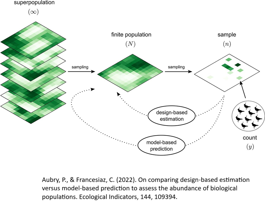
Design-Based

• the values themselves are held to be fixed, whereas the sampling process is random.

Design-Based

• Key Strengths: the population of interest is often defined (e.g., grid area); does not relying on stochastic models representing the structure of the data for reliable inference

• Key Weaknesses: limited in application; still requires models to accommodate observational processes, such as detection probability

Design-Based

• \(\textbf{Y}\) = [\(y_1\),…,\(y_N\)]

• \(\textbf{u}\) = [\(y_1\),…,\(y_n\)]

Design-Based

• \(\textbf{Y}\) = [\(y_1\),…,\(y_N\)]

• The population mean is \(\bar{Y} = \sum_{i=1}^N Y_i / N\) and the sample mean is \(\hat{\bar{y}} = \sum_{i=1}^n y_i / n\)

• The population mean describes ….?

• \(\textbf{y}\) is a random vector that has \(n\) random values One sample of 4 cells.

\(\boldsymbol{y} = \begin{matrix} [y_{1} & y_{2} & y_{3} & y_{4 }]\end{matrix}\)

\(\boldsymbol{y}' = \boldsymbol{y}^{T} = \begin{bmatrix} y_{1} & \\y_{2} &\\ y_{3} & \\y_{4 }\end{bmatrix}\)

Random Variable

Wikipedia: A random variable (also called ‘random quantity’ or ‘stochastic variable’) is a mathematical formalization of a quantity or object which depends on random events.

We observe samples from the domain or population or sampling frame.

Samples are observed with some probability.

Statistic

• \(\hat{\bar{y}}\) is a ‘statistic’ (# computed from a sample) and is also a random variable

• statistics have a sampling distribution, describing the probability associated to observing different values of the statistic

Design-Based Code

TRUTH

#random discrete uniform sampler
rdu<-function(n,lower,upper){sample(lower:upper,n,replace=TRUE)}

mat = matrix(rdu(25, 
                 lower = 0, 
                 upper = 400
                 ),
             nrow=5, ncol=5
             )
mat

     [,1] [,2] [,3] [,4] [,5]
[1,]  253   34  131  168  309
[2,]  259   14  102  110  396
[3,]  326  296  222  261  178
[4,]  253  303  204  255   16
[5,]  355  247    2   13  108

Design-Based Code

Random Sampling

  n = 10
  y = sample(
             c(mat),
             10, 
             replace = TRUE
             )
  y

 [1] 326 178 253 396   2 296   2 247 108 303

Estimator for the population mean

  mean(y)

[1] 211.1

Design-Based Code

Sampling Distribution

# How many ways can we uniquely sample 10 things from 25
combs = function(n, x) {
  factorial(n) / factorial(n-x) / factorial(x)
}

combs(25, 10)

[1] 3268760

Design-Based Code

Get Every combination and then calcualte the mean for each sample of 10

  set.seed(5435)
  all.combs = utils::combn(c(mat), 10)
  dim(all.combs)

[1]      10 3268760

  mean.all.combs = apply(all.combs,2,mean)

Design-Based Code

OR, we can sample enough times to approximate it

  set.seed(5435)
  sim.sampling.dist=replicate(2000,
                              sample(c(mat),10)
                              )
  dim(sim.sampling.dist)

[1]   10 2000

  mean.samples = apply(sim.sampling.dist,2,mean)

Design-Based Code

Model-Based

Inference relies on …

“a statistical model describing how observations on population units are thought to have been generated from a super‐population with potentially infinitely many observations for each unit;” Williams and Brown, 2019

“The analysis need not account for sampling randomization, because the sample is considered fixed. However, the unit values are considered random.” Williams and Brown, 2019

Model-Based

BUT….

when linking ‘unit values’ in a model, we need to account for their dependence.

Randomization allows us to make conditional independence claims among data in our sample, thus the model is simpler.

\(P(y_{2}|y_{1}) = P(y_{2})\)

Model-Based

• Key Strengths: Very flexible. Modeling is magic.

• Key Weaknesses: 1) Can be difficult to assess assumptions and 2) sampling frame is not always clear and thus the population you are infering to is not entirely clear

Model-Based

• \(\textbf{y} \sim\) Poisson(\(\lambda\)) Wikipedia link

• \(y_{i} \sim\) Poisson(\(\lambda\))

• \(\lambda\) is the population mean and variance

• Sample mean Estimator \(\hat{\lambda} = \sum_{i=1}^n y_{i}/n\)

• Maximum-Likelihood Estimate (MLE)

Model-Based Code

#Create a function, to be replicated
  lambda=200
  n.sim=500
  mat.fn = function(lambda){matrix(rpois(25, lambda=lambda),
                               nrow=5, ncol=5
                               )
  }

Model-Based Code

# repeat the function n.sim times
  list.mat = replicate(n.sim, 
                       mat.fn(lambda), 
                       simplify=FALSE
                       )
  length(list.mat)

[1] 500

#One realization
  list.mat[[1]]

     [,1] [,2] [,3] [,4] [,5]
[1,]  213  221  202  204  173
[2,]  195  182  193  190  215
[3,]  221  216  187  182  179
[4,]  176  196  218  210  211
[5,]  218  182  193  229  188

# Sample mean for the first realization
  mean(list.mat[[1]])

[1] 199.76

Model-Based Code

Sampling Distribution

lambda.hat = unlist(lapply(list.mat,FUN=mean))

Statistical Bias

the difference b/w the true value and the mean of the sampling distribution of all possible values; applies to design- and model-based sampling

Statistical Bias (Code)

# Bias
  mean(lambda.hat) - lambda

[1] 0.00544

# relative bias
  (mean(lambda.hat) - lambda)/lambda

[1] 2.72e-05

Precision of the mean (Code)

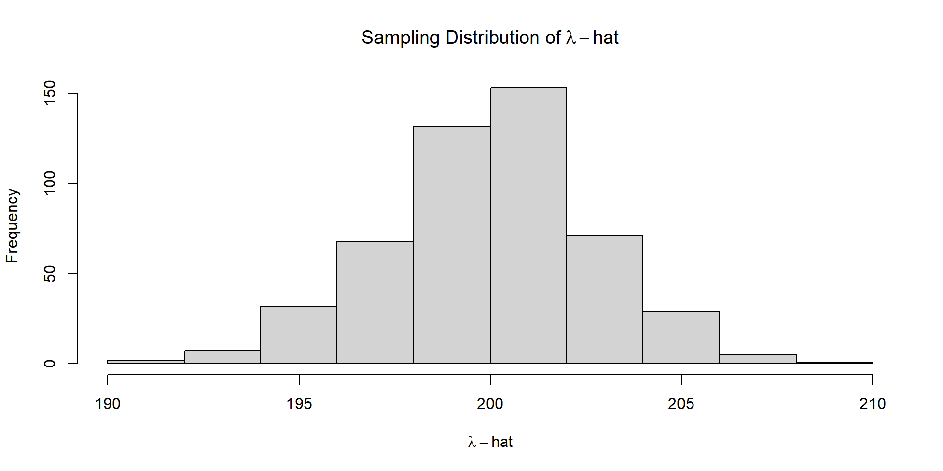
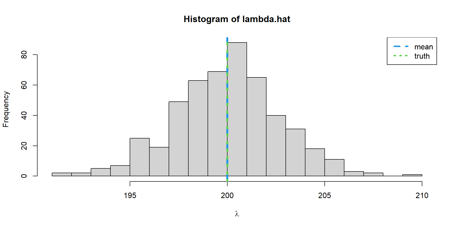
What is the probability that we will observe a mean within 5% of the truth?

We can calculate this using Monte Carlo integration

  diff = 0.025*lambda
  diff

[1] 5

  lower = lambda-diff
  upper = lambda+diff

  index = which(lambda.hat>=lower & lambda.hat <= upper)

#Probability of getting a mean within 5% of the truth
  length(index)/n.sim

[1] 0.934

Take-Aways

1. Study Objectives, Hypotheses, and Predictions

2. Big Data and Sampling

3. Inference and Prediction

4. Model-Based vs Design-Based Inference

Lab

Objectives

• Introduce R Markdown

• Use simulation and design-based sampling to investigate bias and precision

Lab Setup

Let’s add some more reality in our work while using design-based sampling in R.

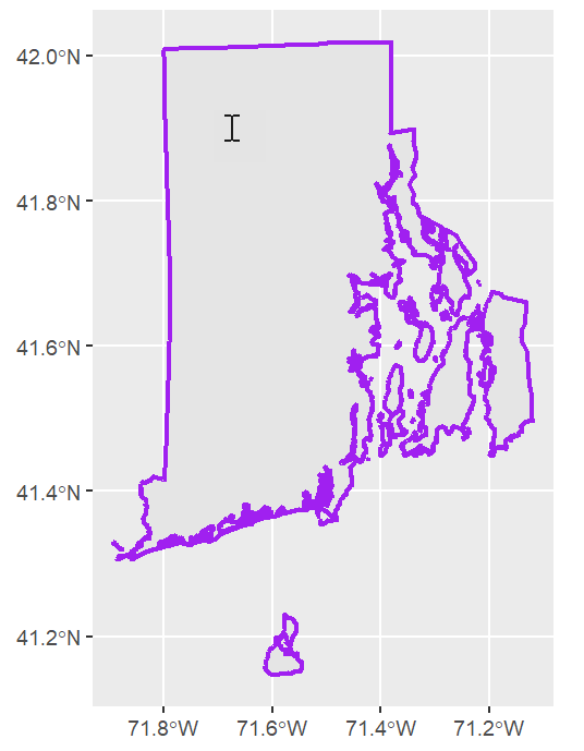
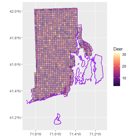
Objective: Evaluate sample size trade-offs for estimating white-tailed deer abundance throughout Rhode Island.

Methodology: Count deer in 1 sq. mile cells using FLIR technology attached to a helicopter.

Lab Setup

Steps to consider

• Sampling Frame

  • all of RI or some subset

Lab Setup

Steps to consider

• “Truth”

  • how many deer per cell; how variable

Lab Setup

Steps to consider

• Sampling Process

  • how to pick each cell

Lab Setup

Steps to consider

• Estimation Process

  • estimate total deer population from the sample

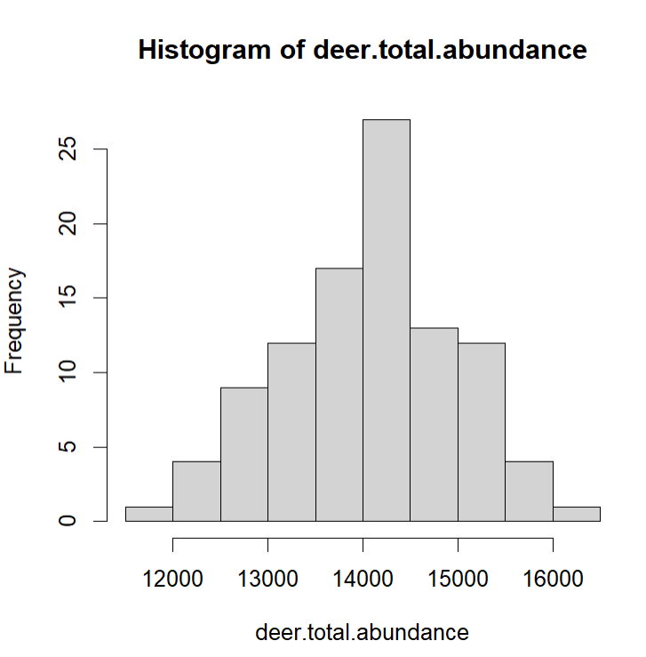
• Criteria to Evaluate

  • use sampling distribution of deer abundance estimate or some other statistic
    

Go to code