Multi-Stage

Multi-Stage Sampling

A key fundamental difference from SRS, stratified, or cluster sampling

But also no new principles.

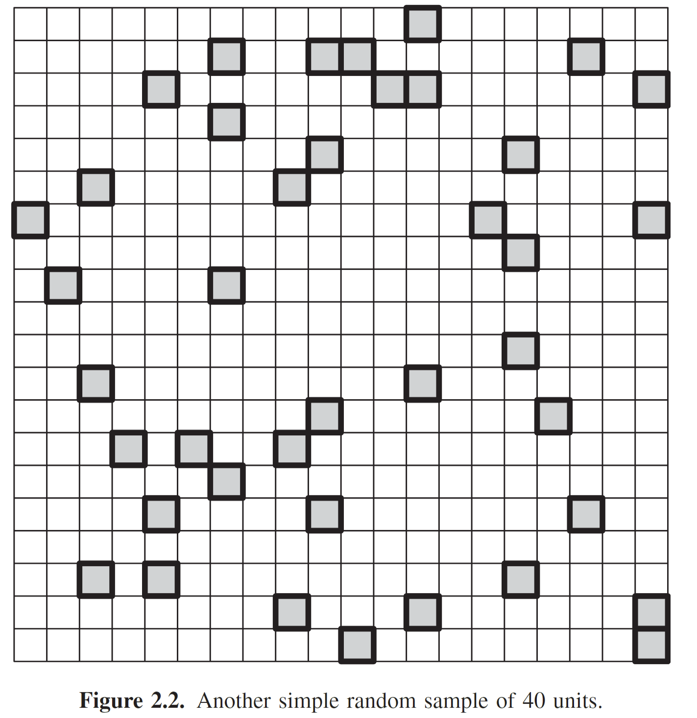
SRS

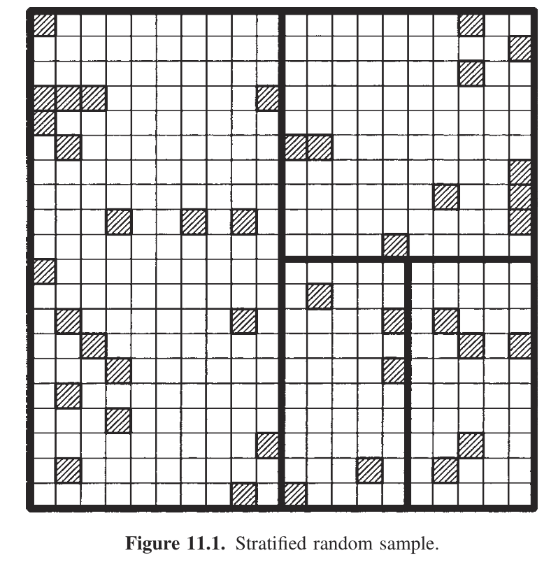
Stratified Sampling

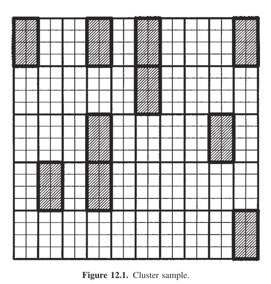
Cluster Sampling

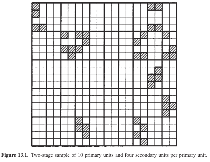
Two-Stage Sampling

Simplest multi-stage

Two-Stage Sampling

Simplest multi-stage

• 1st stage: sample \(n\) primary units (\(N\) = 50; n = 10)
• 2nd stage: for \(i^{th}\) primary unit, select \(m_i\) secondary units (\(M_i = 8; m_{i} = 4\))

Two-Stage Sampling

Simplest multi-stage

• If sampled all \(M_i\) then it is what type of sampling?

Two-Stage Sampling

Simplest multi-stage

We have two-levels of sampling variation!

• Sampling variation of primary units
• Sampling variation of secondary units within primary units

Multi-Stage Sampling

A generalization of cluster sampling in which selection occurs in two or more successive stages.

• Rather than drawing a sample directly from the population, units are chosen in stages
  • larger primary sampling units (PSUs) are selected first, and then
  • smaller secondary sampling units (SSUs) are then sampled within them

Multi-Stage Sampling

Allows flexibility

How though?

Multi-Stage Sampling

Cost is complexity

• need to consider multiple levels of variance estimates

Example

State of Colorado

• National Forests in CO (PSU)
  • Forest mgmt units (SSU)
    • measure course woody debris

Example

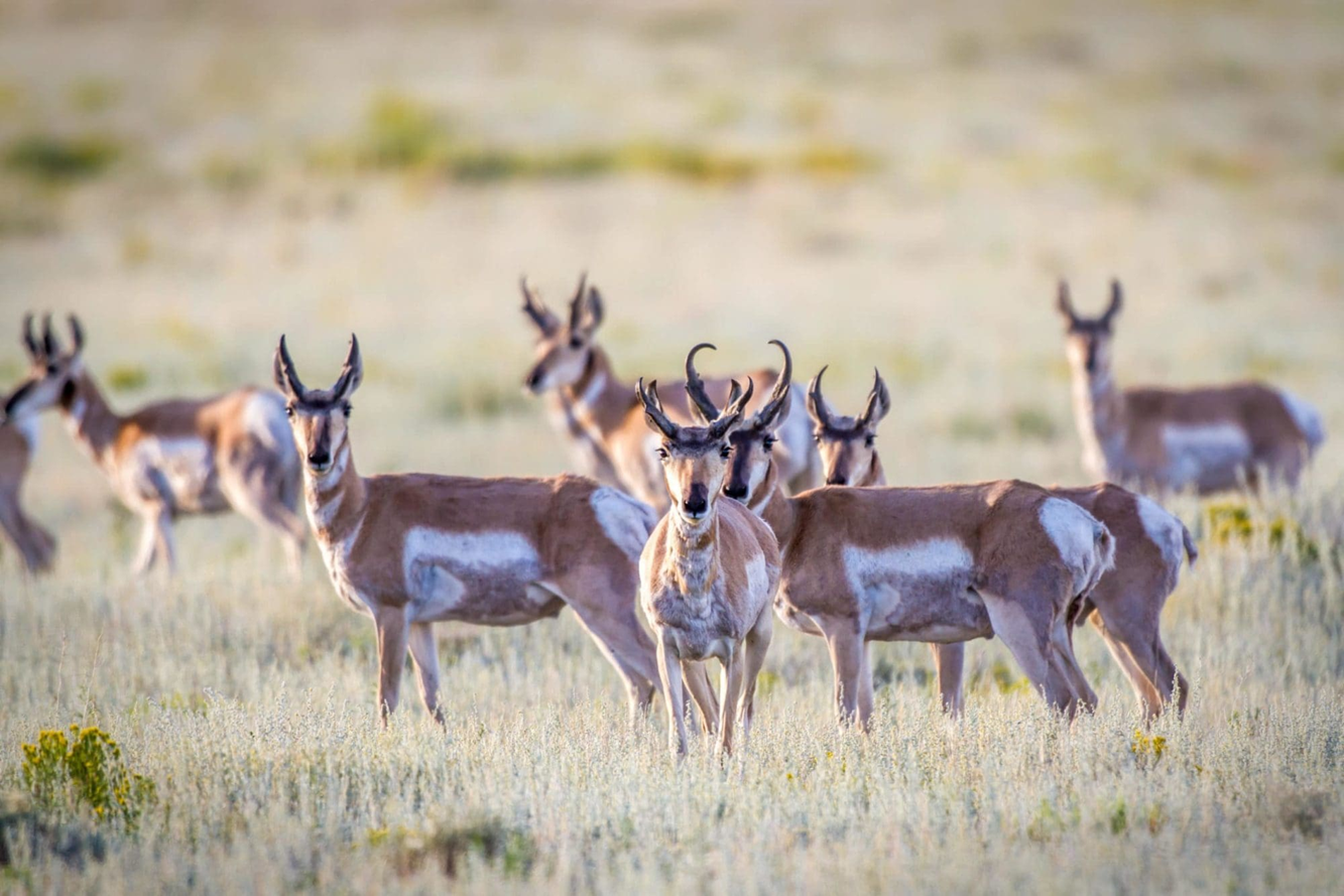
Western U.S. Grasslands/Praries/Shrublands

• Pronghorn Populations (PSU)
  • Individuals (SSU)
    • Scat (Tertiary SU)
      • Measure forb contents in each scat

Examples

Your turn!

Selecting PSUs

• SRS: if no prior information is available

• Stratification: if variables of interest are available (area, measure of variability of interest) then stratify and sample within each stratum

• Systematic: if variables of interest are available, sort by one of these and apply systematic sampling with a random start

• Probability proportional to size: if each primary unit has a known measure of size of importance (based on variables) select units with probabilities proportional to that

Notation

• \(N\) is the number of PSUs in the population
• \(n\) is the number of PSUs in the sample
• \(M_i\) is the number of SSUs in the \(i^{th}\) PSU
• \(m_i\) is the number of sampled SSUs in the \(i^{th}\) sampled PSU
• \(M = \sum_{i=1}^N M_i\) is the number of SSUs in the population
• \(y_{ij}\) is the value for the \(j^{th}\) SSU in the \(i^{th}\) PSU
• \(\tau = \sum_{i=1}^N \sum_{j=1}^{M_{i}} y_{ij}\) is the population total
• \(\mu = \frac{\tau}{M}\) is the population mean per secondary unit

Mean with SRS

Unbiased total of primary unit \(i\)

• \(\hat{\tau}_{i} = \frac{M_i}{m_i}\sum_{j=1}^{m_i} y_{ij}\)

Unbiased Total Population size

• \(\hat{\tau} = \frac{N}{n}\sum_{i=1}^n M_{i} \hat{\mu}_{i}\)

Unbiased Population Mean Per Primary Unit

• \(\hat{\mu} = \frac{\hat{\tau}}{N}\)

Variance of total population size

partitioning the variance in the nested components

\[ \sigma^2_{\hat{\tau}} =\\ \left(N(N-n)\frac{\hat{\sigma}^2_{\text{Between_PSU}}}{n}\right)\\ + \\\left(\frac{N}{n}\sum_{i=1}^n M_{i}(M_{i}-m_i)\frac{\hat{\sigma}^2_{\text{Within_PSU}}}{m_i}\right) \]

Side-Bar

Same idea in model-based inference

We observe the weight of the \(j^{th}\) individual pronghorn within the \(i^{th}\) population

\[ \begin{align*} y_{ij} &= \beta_0 + \mu_i + e_{ij}\\ \mu_{i} &\sim \text{Normal}(\mu_{\text{pop}}, \sigma_{\text{pop}})\\ \epsilon_{ij} &\sim \text{Normal}(0, \sigma_{\text{indiv}}) \end{align*} \]

This Is a hierarchical model or a random-intercept model

Cost Evaluation

Basic idea is that we get cost savings by this strategy!

It may be easier or less costly to observe the same number of secondary units (\(m\)) in a cluster than spread out, as in SRS.

Thompson (Ch.13.4) Cost Function:

\[ C_{\text{total}} = c_{0} + c_1n+c_2*nm \]

assuming the same \(m_{i}\) for each \(i^{th}\) PSU

• \(c_{0}\): fixed overhead cost
• \(c_{1}\): cost per primary unit selected
• \(c_{2}\): cost per secondary unit selected
• \(n\) is the number of sampled primary units
• \(m\) is the number of sampled secondary units within primary

Minimum variance

Minimum value of \(\sigma^2_{\hat{\tau}}\) is

\[ \begin{align*} m_{\text{optimal}} &= \sqrt(\frac{c_1\sigma^2_w}{c_2(\sigma^2_b - \sigma^2_w/\bar{M)}})\\\\ \sigma^2_b &= \frac{\sum_{i=1}^N(\mu_i-\mu)^2}{M-1}\\ \sigma^2_w &= \frac{1}{N}\sum_{i=1}^{N}\sigma_{i}^2\\ \end{align*} \]

• \(\sigma^2_b\): variance b/w primary units
• \(\sigma^2_w\): mean within primary unit variance
• \(\bar{M} =\) average number of secondary units across PSU

Minimum variance

Minimum value of \(\sigma^2_{\hat{\tau}}\) is

\[ \begin{align*} m_{\text{optimal}} &= \sqrt(\frac{c_1}{c_2}\times \frac{\sigma^2_w}{(\sigma^2_b - \sigma^2_w/\bar{M)}})\\\\ \end{align*} \] What ratio of costs would drive up \(m_{optimal}\)?

Minimum variance

Next, lets ignore costs.

\[ \begin{align*} m_{\text{optimal}}^2 &= \frac{\sigma^2_w}{(\sigma^2_b - \sigma^2_w/\bar{M)}} \end{align*} \]

• How does the between and within variances affect our optimal \(m\)?
• How does M affect our optimal \(m\)?
• Generally, how would you investigation this?

Minimum variance

Re-arranged…

\[ \begin{align*} m_{\text{optimal}}^2 &= \frac{1}{\frac{\sigma^2_b}{\sigma^2_w}- \frac{1}{\bar{M}}} \end{align*} \] - How does the between and within variances affect our optimal \(m\)? - How does M affect our optimal \(m\)?