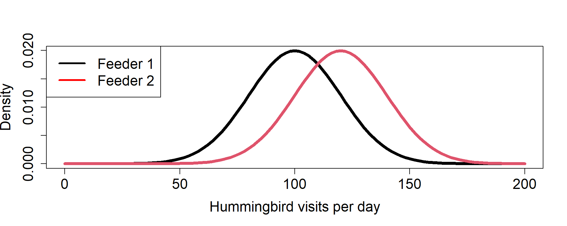
N = 200
d = 10
alpha = 0.01
z = qnorm(1-alpha/2)
sigma2 = 20^2
n = 1/(d^2/(z^2*sigma2)+(1/N))
n
[1] 23.43042
Most common question
Sample size (n) for estimating the population mean (Thompson Ch. 4, Eqn 3)
\[ n = \frac{1}{d^2/(z^{2}\sigma^2)+(1/N)} \]
Objective: to know the average count of bass with fish lice
N = 200
d = 10
alpha = 0.01
z = qnorm(1-alpha/2)
sigma2 = 20^2
n = 1/(d^2/(z^2*sigma2)+(1/N))
n
[1] 23.43042
Thompson Ch.4 : “A bothersome aspect of sample size formulas such as these is that they depend on the population variance”.
. . .
Me - “A bothersome aspect of sample size formulas such as these is that they depend on the difference (\(d\)); we know more about \(n\) than \(d\)”.
. . .
How would you solve this?
. . .
This is a HW question
. . .
Work on problem together OR more about sample sizes?
The null hypothesis testing paradigm is often focused on Type I error (\(\alpha\)), rejecting the null hypothesis when it is actually true.
. . .
The Null hypothesis is commonly, \(H_0(\mu_1 = \mu_2)\)
. . .
Definition: the probability that a test will reject a false null hypothesis.
Type I Error = P(reject \(H_0\) | \(H_0\) is true) = \(\alpha\)
. . .
Power = P(reject \(H_0\) | \(H_1\) is true)
. . .
Power = 1 - Type II Error
. . .
Power = 1 - Pr(False Negative)
. . .
Power = 1 - \(\beta\)
Contributions to statistical power
The statistical test and its assumptions
Effective Sample size (simplest case this is \(n\) per group)
Reality
Objective: To evaluate the relative use of two types of hummingbird feeders.
Null Hypothesis
Mean daily use of each feeder is equal (\(\mu_{1} = \mu_{2}\)).
. . .
Alt. Hypothesis
Mean daily use of each feeder is not equal (\(\mu_{1} \neq \mu_{2}\)).
. . .
Statistical Test: two-tailed t-test
First, we need to define TRUTH
Group1.Mean <- 100
Group1.SD <- 20
Group2.Mean <- 120
Group2.SD <- 20
. . .
library(pwr)
# Wish to test a difference b/w groups 1 and 2
# Want to know if there is a difference in means
#Difference in Means
effect.size <- Group1.Mean-Group2.Mean
#Group st. dev
group.sd <- sqrt(mean(c(Group1.SD^2,Group2.SD^2)))
#Mean difference divided by group stdev
#How does the numerator and denominator influence this number?
d <- effect.size/group.sd
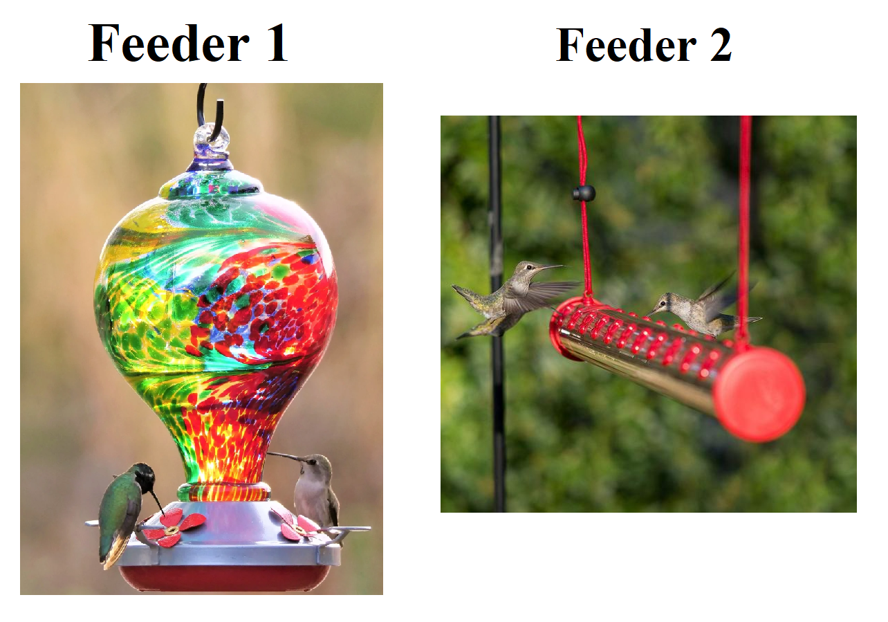
power = 0.8
out = pwr.t.test(d=d,power=power,type="two.sample",
alternative="two.sided")
#Sample Size Needed for each Group
out$n
[1] 16.71472
. . .
Assuming Independence b/w feeders
How do we design our sampling to ensure this?
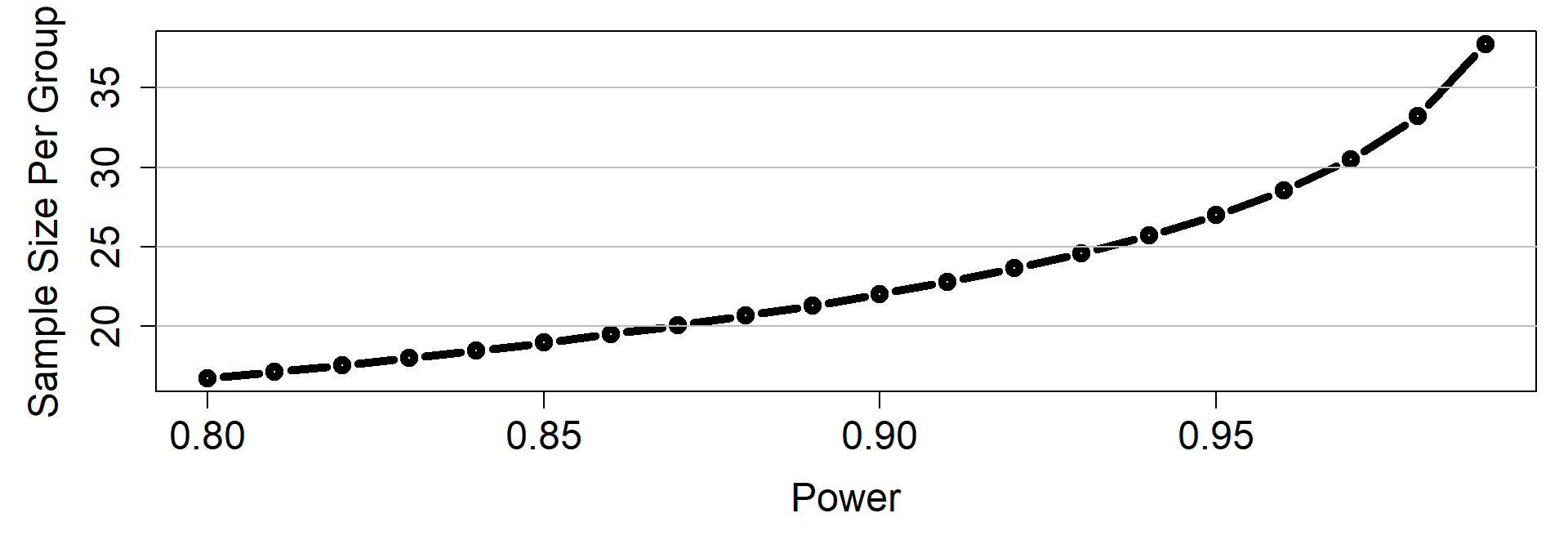
Let’s consider multiple levels of power
. . .
. . .
These results assume we are correct about…
Group1.Mean <- 100
Group1.SD <- 20
Group2.Mean <- 120
Group2.SD <- 20
. . .
What if we are wrong?
How do we evaluate this?
Power, Effect Size, N
# Allow group 1 to vary
Group1.Mean <- seq(10,110,by=5)
#THIS IS THE SAME
Group1.SD <- 20
Group2.Mean <- 120
Group2.SD <- 20
group.sd <- sqrt(mean(Group1.SD^2,Group2.SD^2))
# Variable effect.size
effect.size <- Group1.Mean-Group2.Mean
d <- effect.size/group.sd
#setup combinations of d and power
power = seq(0.8,0.99,by=0.01)
power.d = expand.grid(power,d)
power.d$Var1 = as.numeric(power.d$Var1)
. . .
#make new function and use mapply
my.func = function(x,x2){
pwr.t.test(d=x2,power=x,
type="two.sample",
alternative="two.sided"
)$n
}
# mapply function
out= mapply(power.d$Var1,power.d$Var2, FUN=my.func)
# unstandardized the effect size back to difference of means
power.d$Var2=power.d$Var2*group.sd
out2=cbind(power.d,out)
colnames(out2)=c("power","d","n")
Power, Effect Size, N