Ratio Estimation
(precise auxillary information)

Auxillary Information

stratification used coarse aux. information to improve estimator precision
- groupings
Can we use continuous aux. information?
- Ratio Estimator

Fundamental Information

We sample via probabilistic sampling and observe our primary variable of interest (\(y_i\))
We also record a secondary variable - that correlates with the primary (\(x_i\))
We also know the true population mean/total for the secondary variable (\(\mu_x\))

Is this useful to us??

Relevant Wildlife/Fish/Habitat studies???

Example

We take morphometric data on all Lowland Tree Kangaroos in a forest of Papua New Guinea (6 individuals).

However, what if you end up releasing 2 individuals before getting their weight, but all individuals height was measured.

What was the mean weight of all individuals in the forest?

Example (truth)

Indiv	height	weight
1	32	25
2	24	20
3	28	26
4	20	13
5	36	33
6	25	26

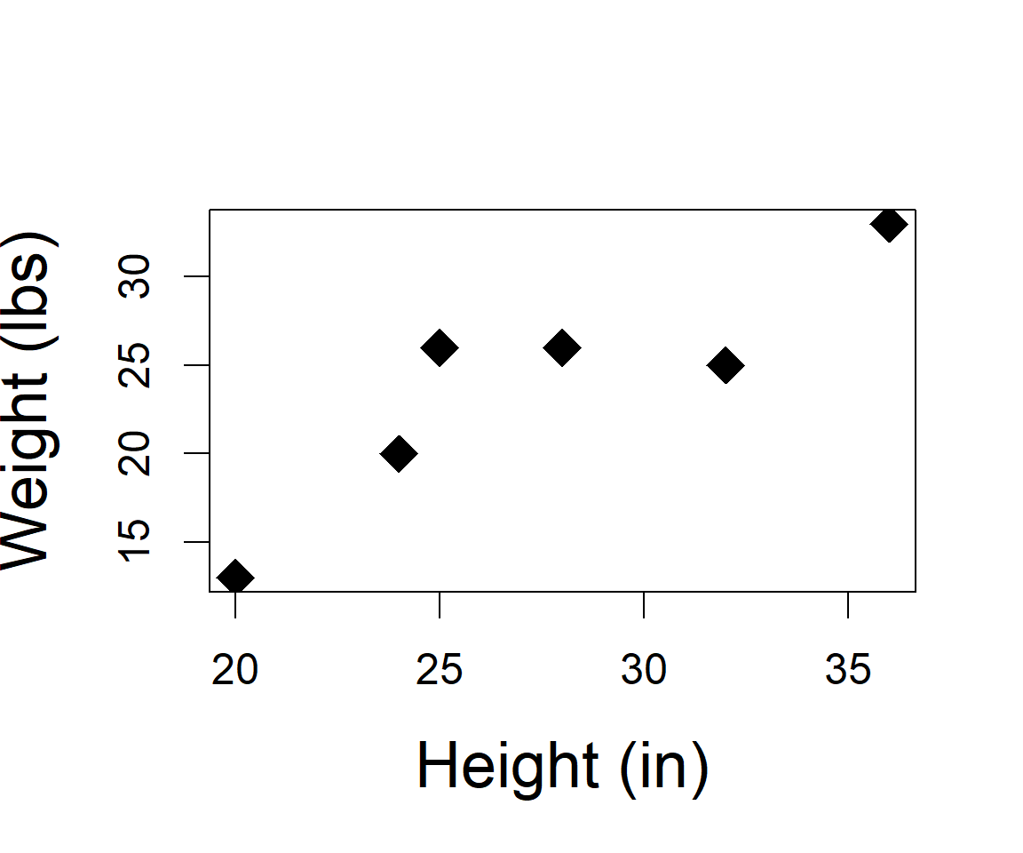
\(\mu_{weight} =\) 23.8333333

\(\mu_{height} =\) 27.5

Example (samples)

Weight

Sample.Number	Indiv.1	Indiv.2	Indiv.3	Indiv.4	means
1	25	25	25	25	25.00
2	25	25	25	25	25.00
3	25	25	20	20	22.50
4	20	20	26	20	21.50
5	20	20	20	20	20.00
6	20	26	26	26	24.50
7	13	26	26	26	22.75
8	13	13	26	26	19.50
9	26	13	13	33	21.25
10	13	13	33	33	23.00
11	13	13	33	33	23.00
12	33	13	33	26	26.25
13	33	26	26	33	29.50
14	26	26	26	33	27.75
15	26	26	26	26	26.00

\(E[\hat{\mu}_{weight}] =\) 23.8333333 \(=\mu_{weight}\)

\(E[\hat{\sigma}^2] = 3.3777\)

Example (samples)

Height

Sample.Number	Indiv.1	Indiv.2	Indiv.3	Indiv.4	means
1	32	32	32	32	32.00
2	32	32	32	32	32.00
3	32	32	24	24	28.00
4	24	24	28	24	25.00
5	24	24	24	24	24.00
6	24	28	28	28	27.00
7	20	28	28	28	26.00
8	20	20	28	28	24.00
9	28	20	20	36	26.00
10	20	20	36	36	28.00
11	20	20	36	36	28.00
12	36	20	36	25	29.25
13	36	25	25	36	30.50
14	25	25	25	36	27.75
15	25	25	25	25	25.00

\(E[\hat{\mu}_{height}] =\) 27.5 \(=\mu_{height}\)

Ratio Estimator of population mean

\(\hat{\mu}_{r}\) = sample ratio \(\times\) population mean of aux

\(\hat{\mu}_{r}\) = sample primary mean / sample aux. mean \(\times\) population mean of aux . . .

\(\hat{\mu}_{r}\) = \(r \times \mu_{x}\)

\(\mu_{x} = \frac{\sum_{i=1}^N x_i}{N}\)

\(\hat{r} = \frac{\sum_{i=1}^n y_i}{\sum_{i=1}^n x_i} = \frac{\hat{\mu}_{primary}}{\hat{\mu}_{secondary}} =\frac{\hat{\mu}_{weight}}{\hat{\mu}_{height}}= \frac{\bar{y}}{\bar{x}}\)

Ratio Estimator of population mean

\[ \hat{\sigma}^2_{\hat{\mu_r}} = \left(\frac{N-n}{N}\right)\frac{\hat{\sigma}^2_r}{n} \]

\[ \hat{\sigma}^2_r = \frac{1}{n-1}\sum_{i=1}^n\left(y_i-rx_i\right)^2 \]

Example (ratio estimator)

Sample.Number	Primary.Weight	Aux.Height	Ratio
1	32.00	25.00	21.48438
2	32.00	25.00	21.48438
3	28.00	22.50	22.09821
4	25.00	21.50	23.65000
5	24.00	20.00	22.91667
6	27.00	24.50	24.95370
7	26.00	22.75	24.06250
8	24.00	19.50	22.34375
9	26.00	21.25	22.47596
10	28.00	23.00	22.58929
11	28.00	23.00	22.58929
12	29.25	26.25	24.67949
13	30.50	29.50	26.59836
14	27.75	27.75	27.50000
15	25.00	26.00	28.60000

\(E[\hat{\mu}_{r}] =\) 23.8683977 \(\neq\) 23.83333

\(E[\hat{\sigma^2}] = 0.523\) (3.37 using Sample Average Estimator)

Comparisons

Sample average of primary (weight) is unbiased
- min: 19.5
- max: 29.5
- Exp.Var: 3.3777778
Ratio estimator of primary (weight) is biased
- min: 21.484375
- max: 28.6
- Exp.Var: 0.5236118

Considerations

Ratio Estimator

design based
estimators are not unbiased (almost at large sample size; Thompson, Ch. 7)
improves precision
depends on linear correlation b/w primary and auxiliary information
requires: when \(x_i = 0\) then \(y_i=0\); i.e., intercept is zero
rarely do we measure one thing when sampling

Classic Example

Pierre-Simon Laplace

Wanted a census of France in 1802
- Primary: Population Size
- Auxiliary: Births
Had all birth records from church records
Sampled 30 communities and calculated a total of 2,037,615 people with 71,866 births
- 2,037,615/71,866 = 28.35 people per birth
Reasoned he could multiply the population number of births by 28.35 to obtain an estimate of population size.

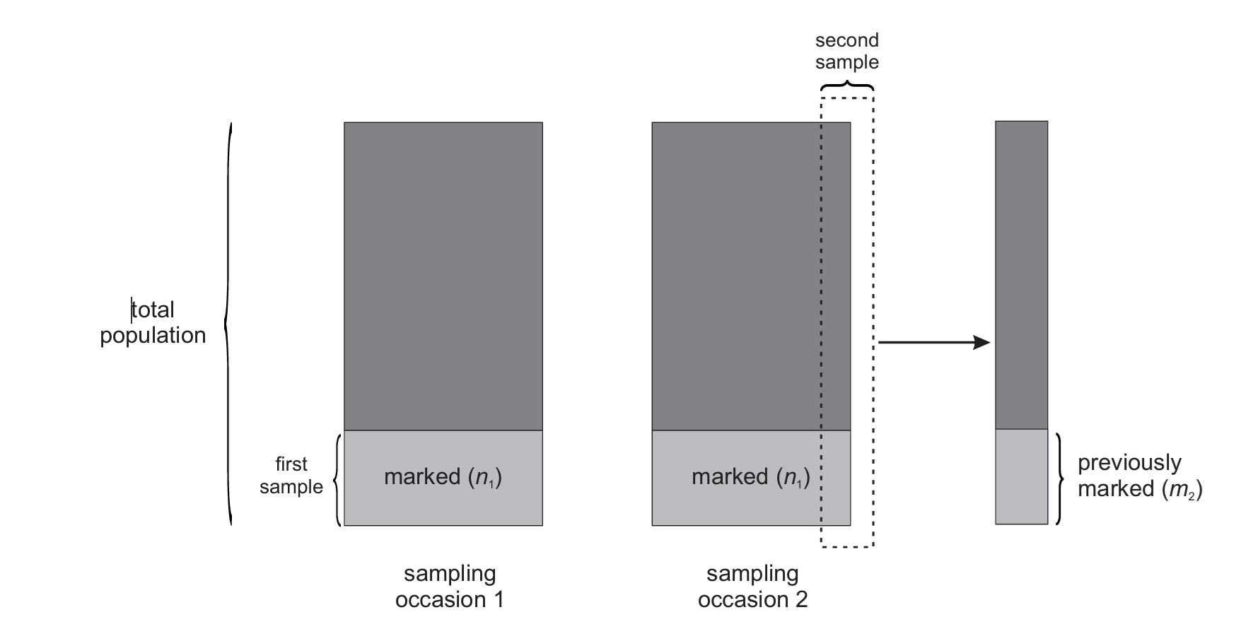
Classic Wildlife Example

Estimating total population

We mark and release \(n_1\) individuals
We go and recapture the same population, catching \(n_2\) individuals
The number of marked individuals caught again is \(m_2\)
Assume equal catchability of individuals and by sample

Classic Wildlife Example

Estimating total population

\[ \frac{m_2}{n_2} = \frac{n_1}{N} \]

Lincoln-Peterson Abundance Estimator

Classic Wildlife Example

\[ \hat{N} = \frac{n_1n_2}{m_2} \]

\[ \hat{N} = \frac{n_1}{\hat{p}} \]

\[ \hat{p} = \frac{m_2}{n_2} \]

Classic Wildlife Example

Model-based Ratio Estimators

\[ \begin{align*} y_{i} &= \beta_0 + \beta_1 \times x_{i} + e_{i}\\ \epsilon_{i} &\sim \text{Normal}(0, \sigma) \end{align*} \]

\[ \begin{align*} E[y_{i}] &= \beta_0 + \beta_1 \times x_{i} \end{align*} \]

Model-based Ratio Estimators

Thompson, Section 8.3:

“Like the ratio estimator, the regression estimator is not unbiased in the design sense under simple random sampling.”

“That is, viewing the y and x values as fixed quantities, the expected value, over all possible samples, of the regression estimator of the population mean of the y’s does not exactly equal the true population mean.”

Unbiasedness Evaluation

# Setup
  N = 500
  set.seed(453543)
  x = rpois(N, 500)

# Fixed 
  beta0 = -5
  beta1 = 4
  sigma = 100

# Random variation- inducing some not perfect correlation
  set.seed(1453543)
  epsilon = rnorm(N, 0, sigma)

# Derive y  
  y = beta0 + beta1*x + epsilon
  

# True population mean
  mean(y)

[1] 1984.943

Unbiasedness Evaluation

Estimators

\[ \begin{align*} \hat{\mu} =& a + b\times\mu_x\\ \hat{\mu}_{y} =& \beta_0 + \beta_1\times\mu_x \end{align*} \]

Thompson, Section 8.1 (ordinary least squares)

\[ \begin{align*} \beta_1 =& \frac{\sum_{i=1}^{n}(x_i-\bar{x})\times(y_i-\bar{y})}{\sum_{i=1}^n(x_i-\bar{x})^2}\\ \beta_0 =& \bar{y}-\beta_1\times\bar{x} \end{align*} \]

Unbiasedness Evaluation

nsim = 10000
pred.model.coef = beta1.save = save.mean=rep(NA, nsim)


for(i in 1:nsim){
  
# Sample size
  n = 100  
  
  #simple random sample
  index = sample(1:N,n)
  
  #Eqns in Section 8.1
  beta1.save[i] = sum((x[index]-mean(x[index]))*(y[index]-mean(y[index])))/sum((x[index]-mean(x[index]))^2)
  beta0 = mean(y[index]) - beta1.save[i] * mean(x[index])
  save.mean[i] =  beta0 + beta1.save[i]*mean(x)
  
  pred.model.coef[i] = coef(lm(y[index]~x[index]))[2]
  
}

Unbiasedness Evaluation

Slope Estimator

hist(beta1.save,breaks=25)
abline(v=beta1,lwd=3,col=2)

mean(beta1.save)-beta1

[1] -0.3461886

Unbiasedness Evaluation

Slope Model

hist(pred.model.coef,breaks=25)
abline(v=beta1,lwd=3,col=2)

mean(beta1.save)-beta1

[1] -0.3461886

Unbiasedness Evaluation

Population Average

hist(save.mean)
abline(v=mean(y),lwd=3,col=2)

mean(save.mean)-mean(y)

[1] 0.1165331

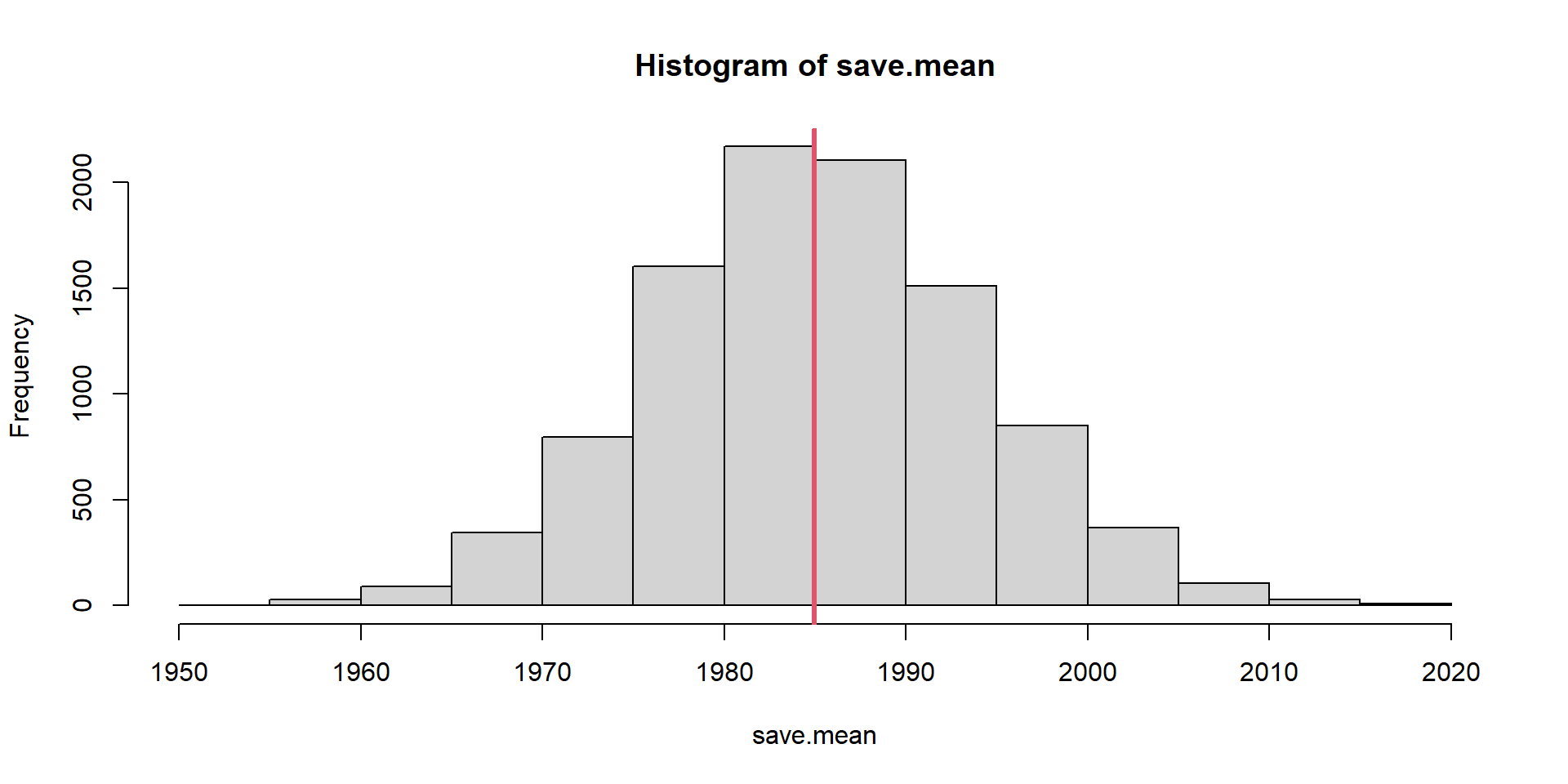
Unbiasedness Evaluation

Slope estimates are not unbiased. Not Design-Unbiased!

What about model-unbiased?

Model Unbiasedness Evaluation

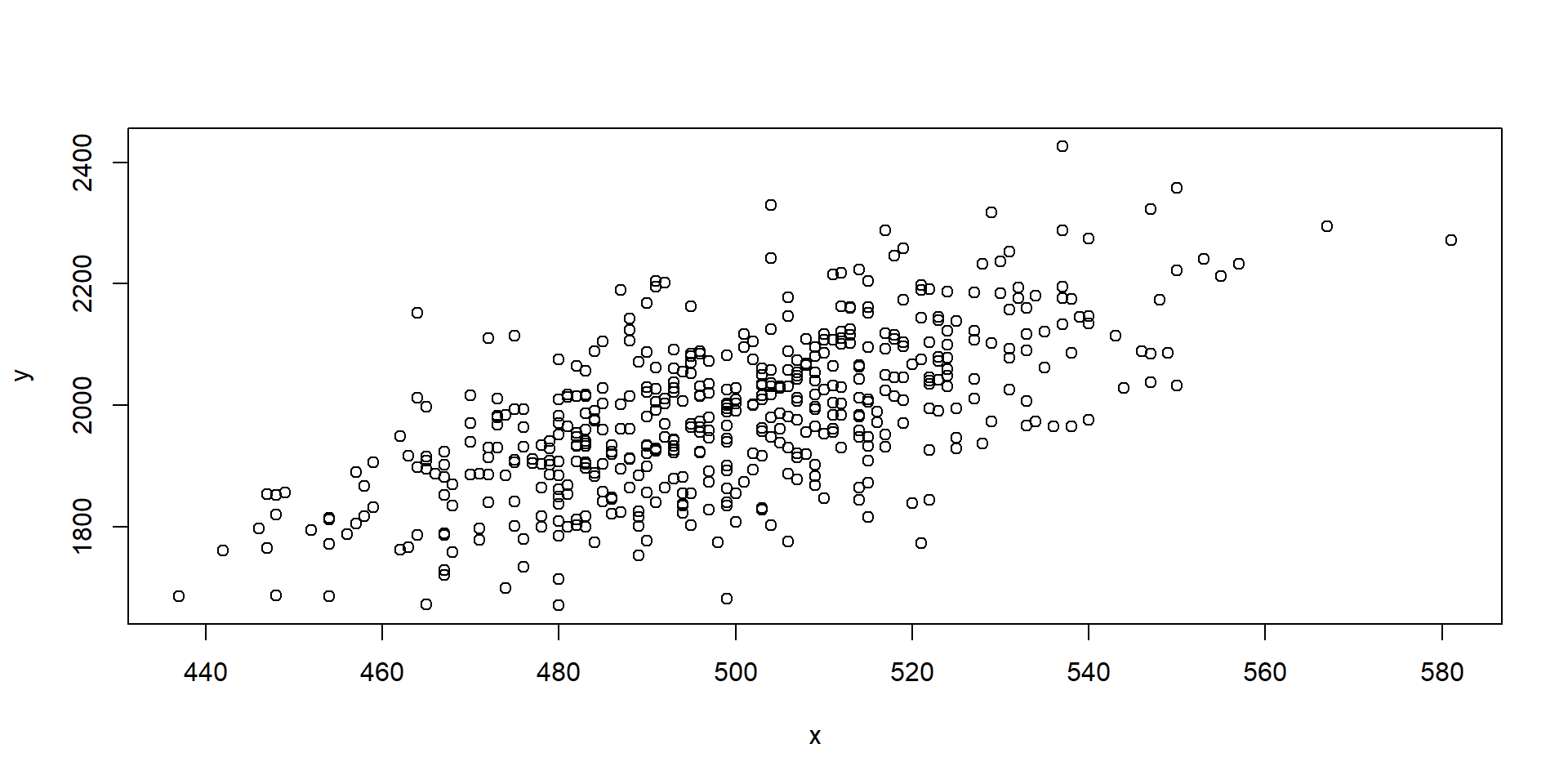
nsim=10000
pred.model.coef= beta1.save = save.mean=rep(NA, nsim)

 N = 500
  set.seed(453543)
  x = rpois(N, 500)

# Fixed 
  beta0 = -5
  beta1 = 4
  sigma = 100


  

for(i in 1:nsim){

# True is now changing!    
  epsilon = rnorm(N, 0, sigma)
  y = beta0 + beta1*x + epsilon

# Sample size
  n = 100  
  
# simple random sample
  index=sample(1:N,n)
  
# Eqns in Section 8.1
  beta1.save[i] = sum((x[index]-mean(x[index]))*(y[index]-mean(y[index])))/sum((x[index]-mean(x[index]))^2)
  beta0 = mean(y[index]) - beta1.save[i] * mean(x[index])
  save.mean[i] =  beta0 + beta1.save[i]*mean(x)
  
  pred.model.coef[i]=coef(lm(y[index]~x[index]))[2]
  
}

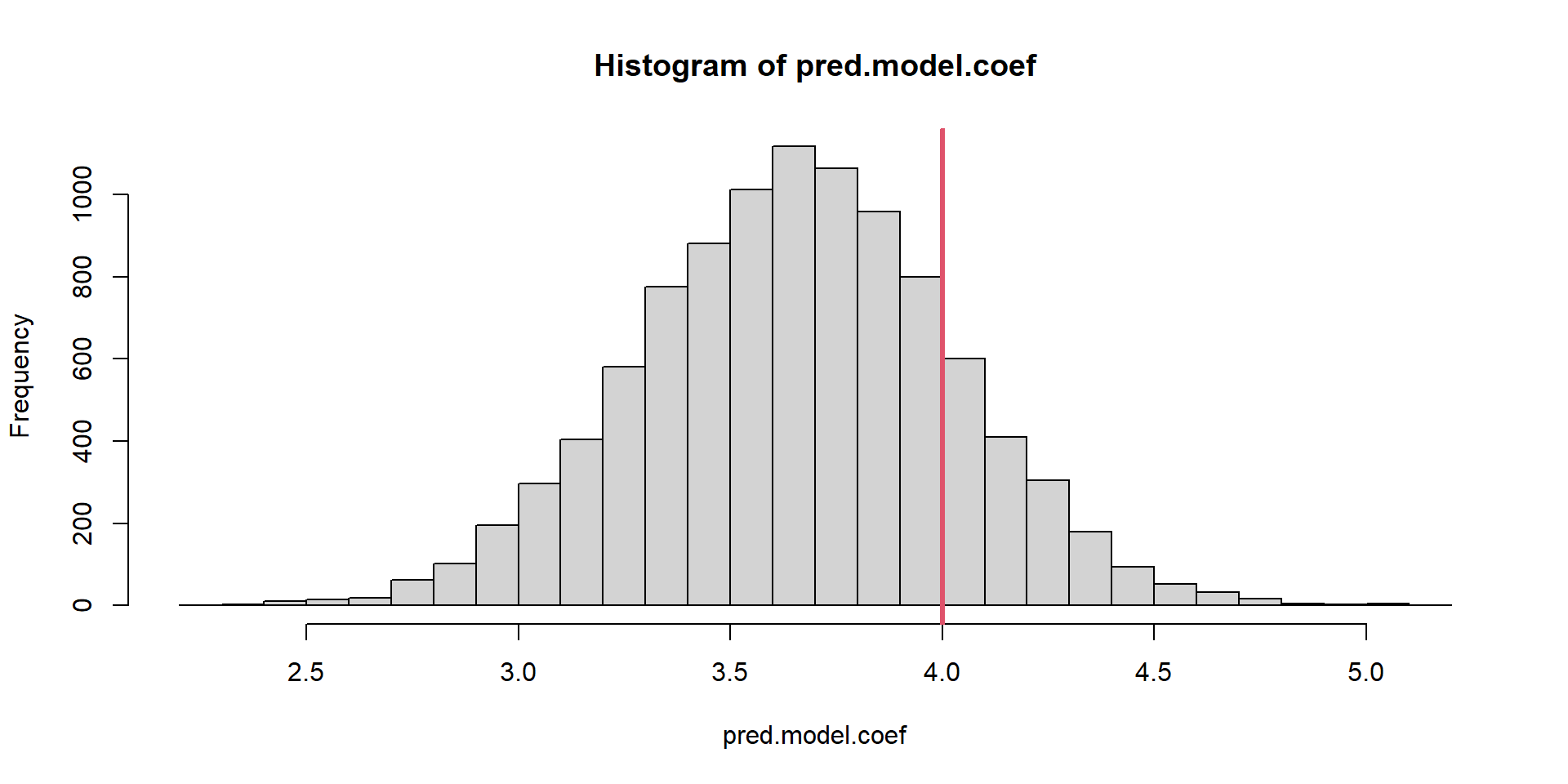
Model Unbiasedness Evaluation

Slope Estimator

[1] 0.0002540056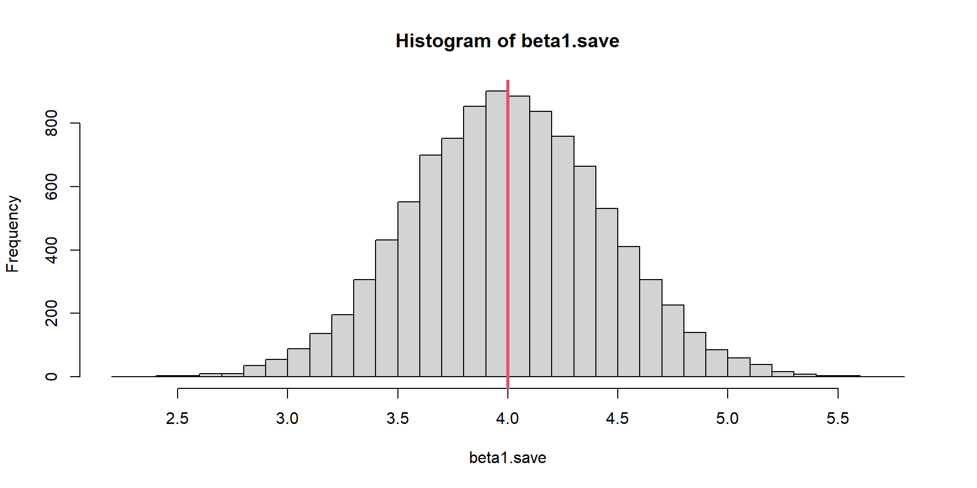

Unbiasedness

“Design unbiased” refers to estimators that are unconditionally unbiased regardless of the underlying model; a very strong assertion!

Some estimators, including Ordinary Least Squares (OLS) may be model unbiased but not design-unbiased.

Unbiasedness

OLS unbiasedness is a property of the estimator for a specific model (super population! the world is not fixed)

Design unbiasedness is a property of the estimator with respect to the design of the sampling, making it model-independent

Ratio Estimation (precise auxillary information)

Auxillary Information

Fundamental Information

Is this useful to us??

Example

Example (truth)

Example (samples)

Example (samples)

Ratio Estimator of population mean

Ratio Estimator of population mean

Example (ratio estimator)

Comparisons

Considerations

Classic Example

Pierre-Simon Laplace

Classic Wildlife Example

Classic Wildlife Example

Classic Wildlife Example

Classic Wildlife Example

Model-based Ratio Estimators

Model-based Ratio Estimators

Unbiasedness Evaluation

Unbiasedness Evaluation

Estimators

Unbiasedness Evaluation

Unbiasedness Evaluation

Slope Estimator

Unbiasedness Evaluation

Slope Model

Unbiasedness Evaluation

Population Average

Unbiasedness Evaluation

Model Unbiasedness Evaluation

Model Unbiasedness Evaluation

Slope Estimator

Unbiasedness

Unbiasedness

Ratio Estimation
(precise auxillary information)